• Photonics Research
  • Vol. 8, Issue 6, 1023 (2020)
Pablo Yepiz-Graciano1, Alí Michel Angulo Martínez1, Dorilian Lopez-Mago2、3、*, Hector Cruz-Ramirez1, and Alfred B. U’Ren1、4、*
Author Affiliations
  • 1Instituto de Ciencias Nucleares, Universidad Nacional Autónoma de México, Apdo. Postal 70-543, Ciudad de México 04510, Mexico
  • 2Tecnologico de Monterrey, Escuela de Ingeniería y Ciencias, Ave. Eugenio Garza Sada 2501, Monterrey, N.L. 64849, Mexico
  • 3e-mail: dlopezmago@tec.mx
  • 4e-mail: alfred.uren@correo.nucleares.unam.mx
  • show less
    DOI: 10.1364/PRJ.388693 Cite this Article Set citation alerts
    Pablo Yepiz-Graciano, Alí Michel Angulo Martínez, Dorilian Lopez-Mago, Hector Cruz-Ramirez, Alfred B. U’Ren. Spectrally resolved Hong–Ou–Mandel interferometry for quantum-optical coherence tomography[J]. Photonics Research, 2020, 8(6): 1023 Copy Citation Text show less
    (a) Simulation of frequency-delay interferogram rc(τ,Ω). (b) Result of integrating the interferogram over Ω, yielding the HOM interferogram. (c) Result of integrating the interferogram over τ, yielding a HOM-like dip in the frequency variable Ω. (d) Fourier transform of (a), so as to yield the time-domain interferogram r˜c(τ,T). (e) Evaluation of r˜c(τ,T) at T=0, yielding the HOM interferogram. (f) Evaluation of r˜c(τ,T) at τ=−1 ps. (g) Function A(Ω). (h) Function B(Ω).
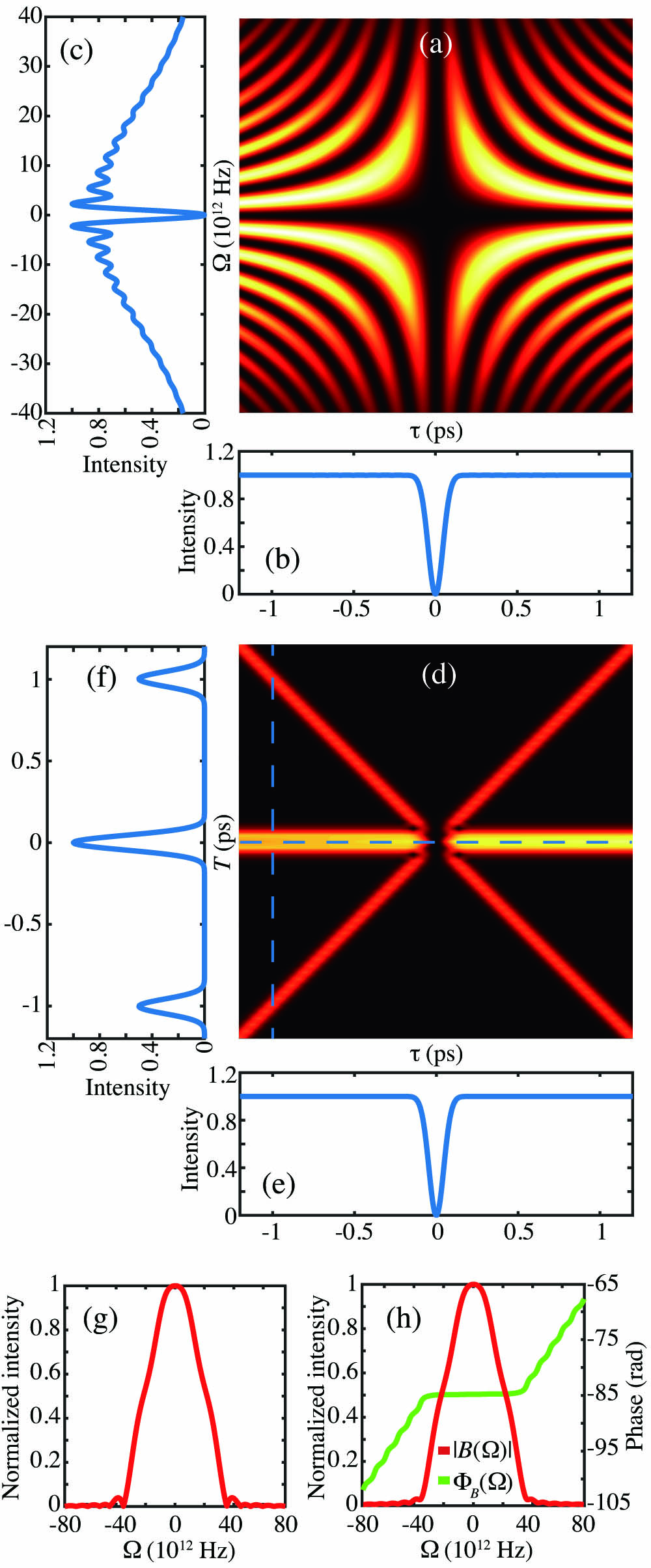
    Fig. 1. (a) Simulation of frequency-delay interferogram rc(τ,Ω). (b) Result of integrating the interferogram over Ω, yielding the HOM interferogram. (c) Result of integrating the interferogram over τ, yielding a HOM-like dip in the frequency variable Ω. (d) Fourier transform of (a), so as to yield the time-domain interferogram r˜c(τ,T). (e) Evaluation of r˜c(τ,T) at T=0, yielding the HOM interferogram. (f) Evaluation of r˜c(τ,T) at τ=1  ps. (g) Function A(Ω). (h) Function B(Ω).
    (a) Frequency-delay interferogram rc(τ,Ω) for two-interface sample (borosilicate coverslip of 170 μm thickness). (b) Result of integrating the interferogram over Ω, yielding the HOM interferogram. (c) Fourier transform of (a) yielding the time-domain interferogram r˜c(τ,T).
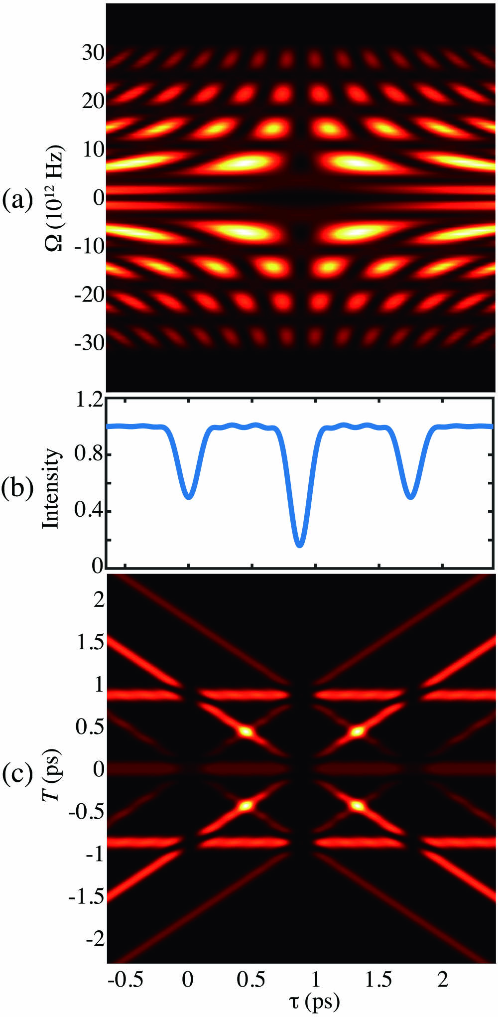
    Fig. 2. (a) Frequency-delay interferogram rc(τ,Ω) for two-interface sample (borosilicate coverslip of 170 μm thickness). (b) Result of integrating the interferogram over Ω, yielding the HOM interferogram. (c) Fourier transform of (a) yielding the time-domain interferogram r˜c(τ,T).
    (a) and (d) Simulation of the temporal-domain interferogram |r˜c(τ,T)| for a three-layer sample (intermediate layer at 40% of the sample thickness, in addition to the two extremal interfaces); in (a) we show the case of an SPDC source centered at 775 nm with a narrowband pump (0.1 nm), while in (d) we increase the pump bandwidth to 10 nm. (b) and (e) Evaluation of |r˜c(τ,T)| at τ0=−1.7 ps; while (b) corresponds to a narrow pump bandwidth (0.1 nm), (e) shows the effect of increasing the bandwidth to 10 nm. (c) and (f) HOM interferogram resulting for the above two cases; (c) for a narrow pump bandwidth (0.1 nm) and (f) for a pump bandwidth of 10 nm.
    Fig. 3. (a) and (d) Simulation of the temporal-domain interferogram |r˜c(τ,T)| for a three-layer sample (intermediate layer at 40% of the sample thickness, in addition to the two extremal interfaces); in (a) we show the case of an SPDC source centered at 775 nm with a narrowband pump (0.1 nm), while in (d) we increase the pump bandwidth to 10 nm. (b) and (e) Evaluation of |r˜c(τ,T)| at τ0=1.7  ps; while (b) corresponds to a narrow pump bandwidth (0.1 nm), (e) shows the effect of increasing the bandwidth to 10 nm. (c) and (f) HOM interferogram resulting for the above two cases; (c) for a narrow pump bandwidth (0.1 nm) and (f) for a pump bandwidth of 10 nm.
    Experimental setup. Ti:Sa, titanium–sapphire laser; TC, temperature controller; L, plano-convex spherical lens; PPLN, periodically poled lithium niobate nonlinear crystal; SF, set of bandpass and long-pass filters; MPC, manual fiber polarization controller; PMC, polarization-maintaining optical circulator; FC, compensating fiber; S, sample; RM, reference mirror; BS, beamsplitter; FSs, fiber spools; TDC, time-to-digital converter; APD, avalanche photodetectors.
    Fig. 4. Experimental setup. Ti:Sa, titanium–sapphire laser; TC, temperature controller; L, plano-convex spherical lens; PPLN, periodically poled lithium niobate nonlinear crystal; SF, set of bandpass and long-pass filters; MPC, manual fiber polarization controller; PMC, polarization-maintaining optical circulator; FC, compensating fiber; S, sample; RM, reference mirror; BS, beamsplitter; FSs, fiber spools; TDC, time-to-digital converter; APD, avalanche photodetectors.
    (a) Experimental measurement of the delay-frequency interferogram rc(τ,Ω), for a single-layer sample (plain mirror). (b) Result of integrating the interferogram over Ω, yielding the HOM interferogram. (c) Result of integrating the interferogram over τ, yielding a HOM-like dip in the frequency variable Ω. (d) Numerical Fourier transform of (a), yielding the time-domain interferogram |r˜c(τ,T)|. (e) Evaluation of |r˜c(τ,T)| at T=0, yielding the HOM interferogram. (f) Evaluation of |r˜c(τ,T)| at τ=−1 ps.
    Fig. 5. (a) Experimental measurement of the delay-frequency interferogram rc(τ,Ω), for a single-layer sample (plain mirror). (b) Result of integrating the interferogram over Ω, yielding the HOM interferogram. (c) Result of integrating the interferogram over τ, yielding a HOM-like dip in the frequency variable Ω. (d) Numerical Fourier transform of (a), yielding the time-domain interferogram |r˜c(τ,T)|. (e) Evaluation of |r˜c(τ,T)| at T=0, yielding the HOM interferogram. (f) Evaluation of |r˜c(τ,T)| at τ=1  ps.
    Reconstruction procedure for the functions A(Ω) and B(Ω), from which we can compute the HOM interferogram through Eq. (6). (a) Evaluation of the delay-frequency interferogram rc(τ,Ω) at τ=−1 ps. (b) Numerical Fourier transform of (a), yielding |r˜c(τ0,T)| with τ0=−1 ps. (c) and (d) Peaks 1 and 2 isolated from |r˜c(τ0,T)| by restricting the T variable to the two windows indicated in panel (b). (e) Function A(Ω) obtained as the inverse Fourier transform of peak 1. (f) Function B(Ω) obtained as the inverse Fourier transform of peak 2, multiplied by the phase exp(iΩτ0); both amplitude and phase are shown.
    Fig. 6. Reconstruction procedure for the functions A(Ω) and B(Ω), from which we can compute the HOM interferogram through Eq. (6). (a) Evaluation of the delay-frequency interferogram rc(τ,Ω) at τ=1  ps. (b) Numerical Fourier transform of (a), yielding |r˜c(τ0,T)| with τ0=1  ps. (c) and (d) Peaks 1 and 2 isolated from |r˜c(τ0,T)| by restricting the T variable to the two windows indicated in panel (b). (e) Function A(Ω) obtained as the inverse Fourier transform of peak 1. (f) Function B(Ω) obtained as the inverse Fourier transform of peak 2, multiplied by the phase exp(iΩτ0); both amplitude and phase are shown.
    Reconstructed HOM dip (red line) and conventional HOM dip obtained through scanning the delay with non-frequency-resolved coincidence counting (black dots).
    Fig. 7. Reconstructed HOM dip (red line) and conventional HOM dip obtained through scanning the delay with non-frequency-resolved coincidence counting (black dots).
    (a) Experimental measurement of the delay-frequency interferogram rc(τ,Ω) for a two-layer sample (borosilicate glass coverslip of 170 μm thickness). (b) Result of integrating the interferogram over Ω, yielding the QOCT interferogram. (c) Numerical Fourier transform of (a), yielding the time-domain interferogram |r˜c(τ,T)|.
    Fig. 8. (a) Experimental measurement of the delay-frequency interferogram rc(τ,Ω) for a two-layer sample (borosilicate glass coverslip of 170 μm thickness). (b) Result of integrating the interferogram over Ω, yielding the QOCT interferogram. (c) Numerical Fourier transform of (a), yielding the time-domain interferogram |r˜c(τ,T)|.
    Reconstruction of the sample morphology and QOCT interferogram for a two-layer sample (borosilicate glass coverslip of 170 μm thickness). (a) Experimental measurement of the function rc(τ0,Ω) at a fixed delay τ0=−0.363 ps. (b) Numerical Fourier transform of (a), yielding |r˜c(τ0,T)|; here we have labeled five of the resulting peaks with the numbers 1–5. (c) Reconstructed QOCT interferogram (red line) and conventional delay-scanning, non-spectrally resolved HOM measurement (black points).
    Fig. 9. Reconstruction of the sample morphology and QOCT interferogram for a two-layer sample (borosilicate glass coverslip of 170 μm thickness). (a) Experimental measurement of the function rc(τ0,Ω) at a fixed delay τ0=0.363  ps. (b) Numerical Fourier transform of (a), yielding |r˜c(τ0,T)|; here we have labeled five of the resulting peaks with the numbers 1–5. (c) Reconstructed QOCT interferogram (red line) and conventional delay-scanning, non-spectrally resolved HOM measurement (black points).
    Pablo Yepiz-Graciano, Alí Michel Angulo Martínez, Dorilian Lopez-Mago, Hector Cruz-Ramirez, Alfred B. U’Ren. Spectrally resolved Hong–Ou–Mandel interferometry for quantum-optical coherence tomography[J]. Photonics Research, 2020, 8(6): 1023
    Download Citation