Abstract
In this paper, we revisit the well-known Hong–Ou–Mandel (HOM) effect in which two photons, which meet at a beamsplitter, can interfere destructively, leading to null in coincidence counts. In a standard HOM measurement, the coincidence counts across the two output ports of the beamsplitter are monitored as the temporal delay between the two photons prior to the beamsplitter is varied, resulting in the well-known HOM dip. We show, both theoretically and experimentally, that by leaving the delay fixed at a particular value while relying on spectrally resolved coincidence photon counting, we can reconstruct the HOM dip, which would have been obtained through a standard delay-scanning, non-spectrally resolved HOM measurement. We show that our numerical reconstruction procedure exhibits a novel dispersion cancellation effect, to all orders. We discuss how our present work can lead to a drastic reduction in the time required to acquire a HOM interferogram, and specifically discuss how this could be of particular importance for the implementation of efficient quantum-optical coherence tomography devices.1. INTRODUCTION
The present work lies at the crossroads of experimental quantum optics and biomedical applications. Advances in quantum technologies have made possible an exciting breadth of applications in fields such as communications [1], imaging [2], and computation [3]. In this work, we aim to explore the application of quantum-optical effects in the field of biomedicine by studying the well-known Hong–Ou–Mandel (HOM) interference effect in an interesting new light. This effect, through which two photons that meet at a beamsplitter can exhibit quantum interference, represents a hallmark of quantum optics. First demonstrated by Hong et al. [4], it relies on the destructive interference that occurs between the reflected–reflected (RR) and transmitted–transmitted (TT) alternatives if these are indistinguishable, leading to null in coincidence counts across the two beamsplitter outputs. It is a remarkable effect that is fundamentally based on the quantum-mechanical nature of the interfering states of light. Recently, HOM interference has been realized using different platforms, including silicon photonics integrated circuits [5] and frequency-domain interferometers [6].
In a typical HOM experiment, the signal and idler photons in a given pair produced by the spontaneous parametric downconversion (SPDC) process reach the two input ports of a beamsplitter with a controllable temporal delay between them. While for sufficiently large delays, the TT and RR alternatives become distinguishable, and the quantum interference is thus inhibited, at zero delay, the well-known suppression of coincidence counts occurs. The resulting coincidences versus delay curve, which we refer to in this paper as the HOM interferogram, then exhibits a characteristic dip centered at zero delay. The dip characteristics can reveal useful information about the quantum state of the interfering photon pairs. If both interfering photons emanate from a single SPDC source, on the one hand, the observed dip visibility quantifies the degree of symmetry in the photon-pair state upon interchanging the roles of the signal and idler photons. On the other hand, the shape of the dip, as is to be described below, substantially corresponds to the Fourier transform of the photon-pair joint spectral amplitude so that the dip width is inversely proportional to the SPDC bandwidth [4]. Therefore, HOM interferometry can be used for photon-pair characterization.
An interesting direct consequence of the destructive interference between the TT and RR alternatives is that the quantum state emanating from the two output ports and of the beamsplitter exhibits path entanglement, in particular representing the NOON state [7]. Such states are attractive because they show the quantum-conferred phase super-resolution effect [8]. Another interesting property of HOM interference is that if the SPDC source used is based on a continuous-wave (CW) pump, the HOM visibility is insensitive to even-order dispersion experienced by one or both photons prior to reaching the beamsplitter [9,10]. This remarkable property led to the proposal of a quantum version of optical coherence tomography (OCT) [11], which is based on a HOM interferometer except that one of the SPDC photons is reflected from a sample under study before reaching the beamsplitter [12]. Under appropriate conditions, a distinct HOM dip can appear for each interface within the sample, thus yielding useful morphological information about such a sample. Interestingly, because the resolution depends on the HOM dip width, this scheme benefits from the dispersion cancellation effect mentioned above: the instrument’s resolution is not affected by even-order dispersion in the sample. In addition, it has been shown that this quantum OCT (QOCT) scheme leads to a quantum-conferred factor of 2 enhancement in resolution as compared to an equivalent classical system with the same bandwidth [13].
Sign up for Photonics Research TOC. Get the latest issue of Photonics Research delivered right to you!Sign up now
Current advances in photodetection technologies and the development of highly efficient SPDC sources have revived the interest in developing efficient QOCT systems [14–16]. A Michelson version of QOCT has been shown to represent a functional and robust configuration, which can benefit from the incorporation of novel photon-number-resolving detectors [17], and is amenable to miniaturization [18,19]. A recent full-field QOCT implementation has been demonstrated by our group using an intensified CCD camera [20]. This method, akin to full-field OCT, reduces considerably the time required for probing a three-dimensional object by eliminating the need for raster scanning the transverse section of the sample. We have developed a fiber-based QOCT system that incorporates spectrally engineered photon pairs in the telecom band. In particular, we have demonstrated interesting interference effects that depend on the type of frequency entanglement [21]. In terms of axial resolution, beyond the quantum-conferred improvement factor of 2, it is possible to incorporate spectral engineering in the form of chirped, aperiodically poled nonlinear crystals to obtain submicrometer resolutions [22,23]; alternatively, a Fisher information analysis can result in attosecond resolutions [24]. Moreover, it is worth mentioning that another optical sectioning technique employing nonclassical light has recently been demonstrated, called induced coherence tomography [25], which relies on the concept of induced coherence between two downconverters to infer the internal structure of the sample [26,27].
While in a typical HOM experiment, the signal and idler photon pairs are detected in a non-spectrally resolved manner, in the present work, we explore the benefits of lifting this restriction and permitting spectrally resolved coincidence photon counting of the optical modes corresponding to the beamsplitter output ports. Other groups have carried out related experiments in which the joint spectral intensity of the output quantum state is analyzed as the delay is varied [28–30]. In this paper, we show both theoretically and experimentally that leaving the delay fixed while enabling spectrally resolved coincidence counting, it becomes possible to recover the HOM interferogram, which would have been obtained through a standard delay-scanning, non-spectrally resolved HOM measurement. We show that this technique permits the recovery of information about the two-photon state with dispersion cancellation to all orders. Importantly, we show that from a single delay value larger than the dip half-width, we are able to extract the HOM dip with the same background level of counts as obtained in the standard measurement based on a sufficiently large number of delay stops for the adequate sampling of the dip structure. The importance of this is that the time required to obtain the HOM interferogram can be drastically reduced. As we discuss below, this fixed-delay HOM scheme can be particularly useful in the context of QOCT, for which the standard delay-scanning approach leads to the need for long acquisition times, which is impractical for real-life conditions, e.g., clinical settings. We hope that this work will pave the way towards the deployment of QOCT as a practical technology.
2. THEORY
The two-photon state produced by SPDC for an incident undepleted CW pump may be written as [31] where is the degenerate SPDC frequency, in terms of the pump frequency , assumed to exhibit a negligible frequency spread, with the pump spectral amplitude modeled as a delta function . We also assume a low parametric gain, so that multiple-pair emission may be disregarded. This state involves the energy-conserving signal and idler frequencies, in terms of a frequency non-degeneracy variable . Here, is a constant related to the conversion efficiency and represents the joint amplitude function given by where is the crystal length, describes an interference filter acting on the signal and idler photons, and is the phase-matching function in terms of the pump , signal , and idler wavenumbers and the poling period (in the case of a periodically poled nonlinear crystal). is a normalization factor, defined so that the integral of over all yields unity.
A standard HOM interference experiment involves the signal and idler photons from an SPDC source being directed into the two input ports of a beamsplitter. The coincidence count rate across the two output ports of the beamsplitter is monitored as a function of the signal–idler delay introduced prior to the beamsplitter. The result is the well-known HOM dip, exhibiting a null in coincidence counts centered at resulting from destructive interference between indistinguishable RR and TT pathways [4]. We will refer to the background level of counts as (i.e., the number of coincidences occurring for , where is the dip width). It has been shown that the standard HOM interferogram can be expressed in terms of and as follows [4]: Note that in the above expression, the background level of counts depends essentially on the flux of the SPDC photon-pair source. Note also that the frequency integral in Eq. (3) corresponds to an experimental situation in which we do not frequency resolve the photons emanating from the HOM beamsplitter output ports. In this paper, we are interested in studying the effect of spectrally resolving these output photons, which corresponds to removing the mentioned frequency integral, thus obtaining a frequency-delay (, ) dependent and normalized interferogram of the form where, evidently, the following relationship between and is obeyed: It is straightforward to expand Eq. (4) to obtain the expression in terms of a frequency-symmetrized, real-valued joint spectral intensity , and a complex-valued cross term , i.e., Clearly, the function has a delay-independent contribution characterized by , as well as a delay-dependent term described by .
In order to illustrate these relationships, we present in Fig. 1 simulations for a specific experimental situation involving a periodically poled lithium niobate (PPLN) crystal pumped by a Ti:sapphire laser operating at 775 nm in CW mode with poling period . Figure 1(a) shows a simulation of the delay-frequency interferogram for this situation, with all simulation parameters corresponding to the experiment described in Section 4 and shown in Fig. 5. As is apparent from Fig. 1(a), the HOM interferogram exhibits an interesting added richness when the output modes from the beamsplitter are frequency-resolved. Note that at , there is a null in coincidence counts along all values. As the value of increases, oscillations along appear, with a linearly decreasing period, proportional to . The function limits the maximum spread of the frequency-delay HOM interferogram along the frequency variable .
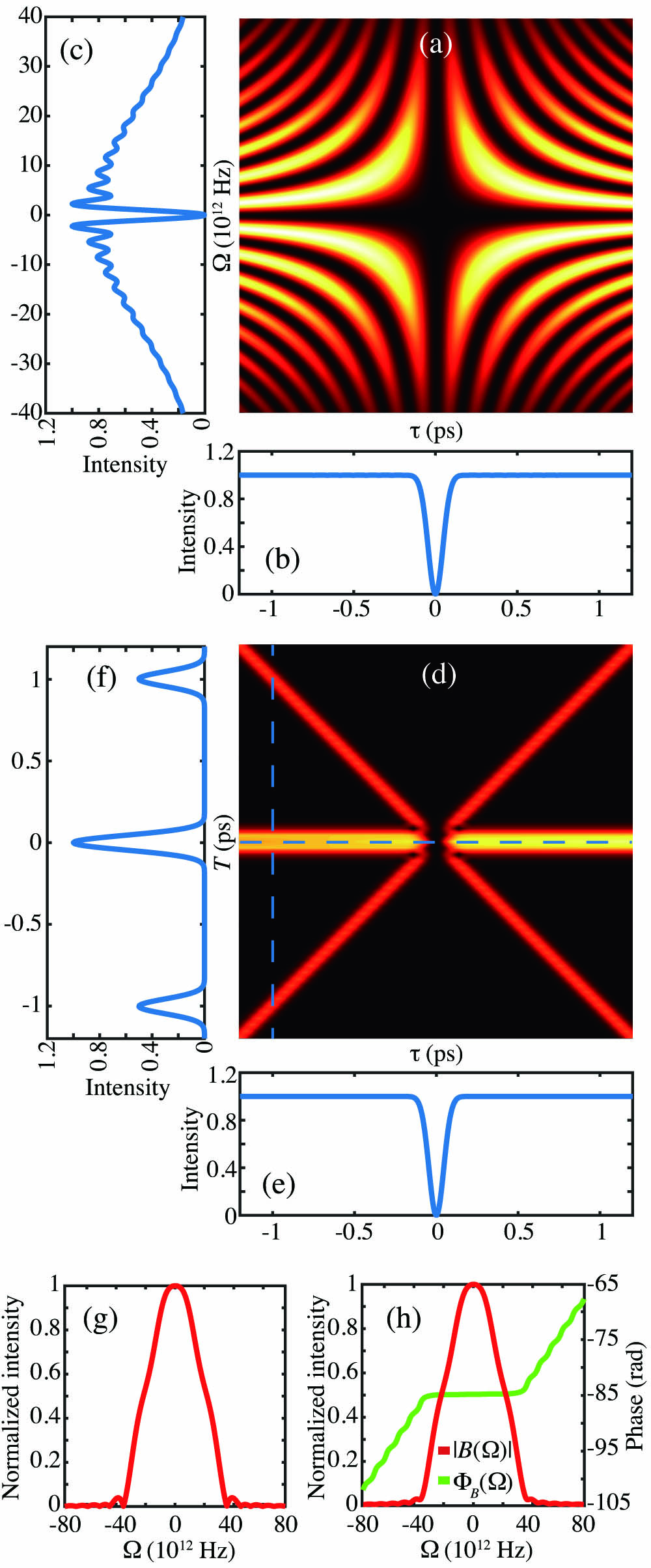
Figure 1.(a) Simulation of frequency-delay interferogram . (b) Result of integrating the interferogram over , yielding the HOM interferogram. (c) Result of integrating the interferogram over , yielding a HOM-like dip in the frequency variable . (d) Fourier transform of (a), so as to yield the time-domain interferogram . (e) Evaluation of at , yielding the HOM interferogram. (f) Evaluation of at . (g) Function . (h) Function .
As is clear from Eq. (5), integrating this frequency-delay interferogram over yields the standard HOM interferogram, as shown for the particular situation of the previous paragraph in Fig. 1(b). An interesting possibility is to integrate over the delay variable instead; we have shown the resulting trace in Fig. 1(c). Physically, this would represent the effect of averaging over all temporal delays, while monitoring the coincidence rate versus the frequency variable . It is interesting that a HOM-like dip also appears versus the frequency variable, with the interpretation that the frequency-degenerate pairs (with ) lead to indistinguishable RR and TT pathways with the effect of destructive interference and a null in coincidence counts. Note that the frequency-delay interferogram of Fig. 1(a) is nearly symmetric in and ; however, is effectively apodized along , reflecting the limited spectral spread of the photon pairs, governed by f(). In fact, we have verified that if the photon pairs are modeled as non-band-limited, the shape of the spectral HOM dip in Fig. 1(c) becomes identical to the more usual delay-dependent dip in Fig. 1(b). Although a detailed discussion of the spectral HOM effect shown in Fig. 1(c) is beyond the scope of this paper, it may be seen from Fig. 1(a) that: 1) the averaging over means that non-zero delays will contribute to the overall destructive interference observed, and 2) for a small bandwidth centered at , a null in coincidence counts occurs for all values of . It is then clear that for non-zero delays (i.e., ), the two photons in a given pair do not temporally overlap in the beamsplitter and, nevertheless, can interfere. In this context, there is a certain parallel with the work of Pittman et al. [32], in which a HOM dip is observed for signal and idler photons that never meet at the beamsplitter.
For the specific case shown in Fig. 1(a), we also show, in Fig. 1(g), a plot of the function , which by construction is symmetric in , and in Fig. 1(h) plots of and . These functions will play an important role below. In order to continue with our discussion, it is helpful to Fourier transform the interferogram in the variable, thus obtaining a 2D time-domain interferogram as follows: in terms of , the Fourier conjugate variable to ; note that because is a real, even function of , is real. Figure 1(d) shows a plot of the function corresponding to the same situation as in Fig. 1(a). It is interesting to point out that the standard HOM interferogram can be obtained by evaluating the 2D time-domain interferogram at , i.e., ; see Fig. 1(e). Furthermore, it is straightforward to show that can be expressed in terms of and , which correspond to the Fourier transform of the functions and , respectively, as Note that the condition [see Eq. (8)] implies that is real. Note also that the HOM interferogram in any of its forms, i.e., , , or , is fully determined by the two functions and . While a standard HOM interferogram is obtained through a non-frequency-resolved coincidence measurement across the two HOM beamsplitter output modes as a function of the delay , we show below that from a frequency-resolved HOM interferogram at a fixed delay, i.e., for , we can extract functions and , and subsequently numerically compute the HOM interferogram , which would have been obtained through a delay-scanning measurement. Importantly, we will show that frequency-resolved HOM data for a single delay value , selected to lie outside of the standard HOM dip so that we have access to the full background level of coincidence counts , contains the same information as a standard delay-based HOM measurement, assuming that the acquisition time per data point is the same in both measurements (a single point for the frequency-resolved measurement versus a collection of points for the standard measurement).
Indeed, for a sufficiently large fixed value of the delay , the resulting time-domain interferogram yields three distinct peaks corresponding to each of the terms in Eq. (10); see Fig. 1(f). By sufficiently large, we mean that the fixed-delay must be larger than the temporal width of each of the three peaks, so that these do not overlap—note that because the peak widths are related to the HOM dip width, this translates into setting the delay to lie outside of the dip. It is notable that from an experimental measurement at a fixed delay , it then becomes possible to extract functions and through the following series of steps: 1) select a value of delay and experimentally obtain the function through a spectrally resolved HOM interferometer, 2) numerically compute Fourier transform, thus obtaining function , 3) numerically filter each of the three peaks in turn, 4) compute a numerical inverse Fourier transform for each of the three peaks, and 5) multiply the result by the delay-dependent phases , 1, and (resulting from the Fourier shift theorem for each of the three peaks, respectively) and complex conjugate the data from the left-hand-side peak, so as to obtain the function in the case of the central peak and the function from any of the two side peaks. In fact, the two side peaks contain duplicate information, and it is thus only necessary to carry out this procedure for the central peak and one of the side peaks. However, in order to take advantage of all coincidence counts (distributed among the three peaks) thus ensuring the best possible reconstruction for a given level of counts, it is helpful to estimate function as the sum of the two side peaks recovered from the procedure above, divided by 2.
The functions and obtained in the manner described in the previous paragraph can then be substituted into Eqs. (6) and (5), so as to numerically compute the standard HOM interferogram . Because all coincidence counts appearing in the standard HOM dip background level are employed in the interferogram reconstruction, and because we utilize Eqs. (6) and (5) (which model the standard HOM effect) in order to predict the interferogram at a fixed delay , the reconstructed and directly obtained interferograms are in fact expected to be equivalent. It is remarkable that at a fixed delay in the background level, i.e., at a delay location exhibiting a flat dependence on and therefore no useful information, enabling a frequency-resolved HOM measurement permits the full extraction of the standard HOM dip.
Let us now address the question of how the resolution of the apparatus used for frequency resolving the photons emanating from the HOM beamsplitter output ports affects the performance of our HOM reconstruction protocol. We know from the Nyquist sampling theorem that for a band-limited function (with maximum frequency component in its spectrum), a sampling period bounded by is sufficient to fully reconstruct the function in question. In our case, the function we wish to determine is , and its spectrum is . Therefore, will be appropriately sampled by a sampling period , where is the location of the side peak with half-width . Disregarding the half-width, i.e., , and letting be the minimum resolvable frequency interval in our apparatus, we arrive at the conclusion that our protocol is able to reconstruct the HOM dip for delays that fulfill Clearly, as the frequency resolution of the apparatus is improved (i.e., as is reduced), we are able to reconstruct a HOM interferogram over a longer stretch of delay values .
3. QUANTUM-OPTICAL COHERENCE TOMOGRAPHY
One of the natural applications for HOM interferometry is QOCT. A QOCT apparatus is closely based on a HOM interferometer, except that one of the SPDC photons is reflected from a sample under study, instead of from a mirror, before reaching the beamsplitter. As is well known, each interface in the sample will produce a HOM dip, along with a cross-interference structure (dip or peak) for each pair of surfaces [21]. In principle, it becomes possible to determine the internal morphology of the sample (number and position of interfaces) from the resulting QOCT interferogram.
Let us consider a hypothetical sample of thickness and index of refraction . The QOCT interferogram will include a HOM dip corresponding to each of the ends of the sample, along with additional dips for possible intermediate interfaces. If the temporal delay for the HOM interferometer is introduced by a displaceable mirror, the two end dips will be separated by a displacement of this mirror. Note that the QOCT resolution is determined by the HOM dip width, which is, in turn, inversely proportional to the SPDC anti-diagonal bandwidth. When carrying out an experimental run, one needs to displace the mirror over the distance with sufficiently small steps so as to be able to determine the location of any possible dips associated with additional interfaces within this range. If the dip width is , or expressed as the required mirror displacement, and if we necessitate points within each dip so as to correctly determine its position, we need a total number of delay stops in the experiment given by As an example, a sample of thickness and index of refraction , with a HOM dip width of and assuming that points per dip are required for the correct identification of all dips, leads to the need for 3000 delay stops (displaceable mirror positions). Assuming that the source brightness is large enough so that an acquisition time of 1 s per point is sufficient, this translates into a total measurement time of 50 min (disregarding the time it takes the motor to move from one position to the next). This leads us to discuss one of the essential challenges for the application of QOCT in practical situations: useful data for an unknown sample often requires experimental runs of long duration, which may be impractical in real-life situations, e.g., in a clinical setting in which the sample could be a human eye. This also leads us to discuss one of the key advantages of our protocol for the reconstruction of a HOM interferogram: for a sufficient frequency resolution (which as was discussed above determines the maximum delay that can be recovered in our reconstruction), comparable data to the standard HOM measurement requiring delay stops [see Eq. (12)] can be obtained with a single delay stop (with the same acquisition time per point). In other words, the reduction factor in the required time for an experimental run can be in the thousands, making this technology potentially much more suitable for real-life situations, including clinical settings.
While discussing the applicability of our work, evidently, three-dimensional sample reconstruction is likely to be needed in most real-life situations. In a recent paper from our group [20], we have demonstrated full-field QOCT (in which we recover the transverse as well as the axial sample structure) by using a triggered intensified CCD camera to detect one of the optical modes following the HOM beamsplitter. It is conceivable to combine spatially and spectrally resolved single-photon detection so as to render our present technique full-field capable.
In terms of the application of our current work to QOCT, let us discuss a two-surface sample, which could be regarded as the simplest possible sample of interest for proof-of-principle purposes. In this case, besides the temporal delay and the variable (Fourier conjugate to ), there is a third temporal variable of interest, the optical thickness of the sample in temporal units, . For simplicity, let us assume that the joint spectrum is symmetric in the sense that , and let us define a new function , along with its Fourier transform . Note that if the joint spectrum is not symmetric, it can be rendered symmetric with an appropriate bandpass filter. We can then show that the time-domain interferogram can be expressed as In Fig. 2(a) we present a plot of the frequency-delay interferogram expected for a two-layer sample that consists of a borosilicate glass coverslip of 170 μm thickness. In Fig. 2(b), we show the QOCT interferogram obtained by integrating over , exhibiting two HOM dips on the sides, each related to one of the two interfaces, as well as the corresponding cross-interference intermediate structure in the center. Note that as is well known, e.g., see Ref. [21], such a cross-interference intermediate structure will appear in the QOCT interferogram for each pair of surfaces in the sample. In Fig. 2(c) we show a plot of the time-domain interferogram , showing for a fixed delay up to nine peaks, as is expected from Eq. (13).

Figure 2.(a) Frequency-delay interferogram for two-interface sample (borosilicate coverslip of 170 μm thickness). (b) Result of integrating the interferogram over , yielding the HOM interferogram. (c) Fourier transform of (a) yielding the time-domain interferogram .
Let us note that the placement of these nine peaks is symmetric; i.e., there is a central peak, and each peak at has a corresponding identical peak at , so that we need only concern ourselves with the central peak along with the four right-hand-side peaks [which appear on the first two lines of Eq. (13)]. Note that the first, third, and seventh terms in the equation are delay-independent, leading to the appearance of three horizontal stripes in Fig. 2(c) (the central one associated with the first term and the two lateral ones associated with the third and seventh terms). The question that we ask ourselves is how to extract morphological information about the sample from an experimental measurement of the function at a fixed delay . In order to answer this question, we remark that the second and fifth terms in Eq. (13) correspond to two peaks, centered at and at , respectively. This implies that the separation between these two peaks directly yields , i.e., the optical thickness of the sample. However, the existence of other peaks can complicate the correct identification of those two peaks, which bear useful information about the sample. Indeed, a major drawback of QOCT with SPDC photon pairs produced by a CW pump is the appearance of an intermediate cross-interference structure (which can be a peak or dip), for each pair of layers in the sample.
In this context, let us also note that the third, fourth, seventh, and eighth terms in Eq. (13) are proportional to . This brings us to refer the reader to an earlier paper from our group [21] in which we studied QOCT in the context of such a two-interface sample, in which we allowed the SPDC pump to be pulsed. In that paper, we show that terms such as these with the argument of the cosine function proportional to the pump frequency will tend to average out to zero as the pump bandwidth is allowed to increase, and can be entirely suppressed if the pump is in the form of a train of ultrashort (fs) pulses. Therefore, for a sufficient pump bandwidth, the peaks associated with the cosine terms are suppressed, leaving only the central peak and the two peaks from which we can extract morphological information about the sample. It turns out that this can be generalized to any number of interfaces: by using a sufficient pump bandwidth, the function exhibits a central peak in addition to one peak per interface (appearing on both sides of the central peak), with the separation between peaks directly yielding the separation between interfaces in the sample. Also, the relative heights of the peaks directly yield information about the relative weights (determined by the reflectivities) of the contributions from each of the interfaces. The downside of using a broadband pump is that dispersion cancellation (see the end of this section for a discussion about dispersion cancellation), for the dispersive phases corresponding to the QOCT sample, no longer occurs. A possible strategy is to use a pump laser that can be switched from femtosecond to CW mode, to first identify those peaks that yield useful morphological information of the sample, and then switch to the CW mode to obtain data with the benefit of dispersion cancellation and with full knowledge of which peaks bear the desired morphological information.
For further illustration of these ideas, let us consider a specific case involving three interfaces; see Fig. 3. Specifically, we assume a sample that contains an intermediate interface at 40% of the total sample thickness of 10 ps in temporal units, as well as the two extremal interfaces. Figure 3(a) shows a plot of the function assuming a CW pump, while Fig. 3(d) shows the same function resulting from a pump with a bandwidth. Note that the plot is significantly simplified, with fewer lines appearing as the pump bandwidth is increased.
Sign up for Photonics Research TOC. Get the latest issue of Photonics Research delivered right to you!Sign up now
Figure 3.(a) and (d) Simulation of the temporal-domain interferogram for a three-layer sample (intermediate layer at 40% of the sample thickness, in addition to the two extremal interfaces); in (a) we show the case of an SPDC source centered at 775 nm with a narrowband pump (0.1 nm), while in (d) we increase the pump bandwidth to 10 nm. (b) and (e) Evaluation of at ; while (b) corresponds to a narrow pump bandwidth (0.1 nm), (e) shows the effect of increasing the bandwidth to 10 nm. (c) and (f) HOM interferogram resulting for the above two cases; (c) for a narrow pump bandwidth (0.1 nm) and (f) for a pump bandwidth of 10 nm.
Let us now select a fixed delay given by . Figure 3(b) shows a plot of the resulting function for a CW pump, where we have chosen not to display the peaks at negative values of on account of the symmetry in this function. In this case, there are 10 peaks for the CW pump case, which are reduced to four peaks for a pulsed pump, a central one, and three additional peaks that directly yield morphological information about the sample.
Note that in the application towards QOCT of our frequency-resolved HOM measurement at a fixed delay , it is not necessary for the determination of the desired morphological information to recover the standard delay-scanning HOM interferogram; i.e., we can directly recover this information from the function at a fixed delay . However, this standard delay-scanning HOM interferogram can be recovered, as we discuss below. We start by rewriting the expression for the HOM interferogram assuming that the function is symmetric, i.e., , for the case in which one of the photons is reflected from a QOCT sample with a response function given by where is the reflectivity of the th interface and is the time traveled in the round-trip from the zeroth layer to the th layer (with chosen to be 0, which corresponds to the positions of all interfaces measured with respect to the position of the first interface).
The HOM interferogram can then be recovered by the following steps: 1) setting a fixed delay and experimentally acquiring the function ; 2) taking a numerical Fourier transform to obtain ; 3) if the SPDC pump has a sufficient bandwidth, taking all peaks appearing on the right-hand side of the central peak and directly obtaining the optical thicknesses from the left-most interface to the th interface from the separation of the peaks, as well as the weight corresponding to each interface from the peak heights, thus constructing the function ; 4) numerically filtering one peak, e.g., the central peak, and taking an inverse Fourier transform, thus obtaining the function ; and 5) numerically computing the HOM interferogram using Eq. (14). In Figs. 3(c) and 3(f) we present the HOM dip recovered using this procedure for a CW pump and a pulsed (with bandwidth) pump. Note that, as expected, for the pulsed pump case, the cross-interference intermediate structures can be fully suppressed.
Let us now discuss the question of dispersion cancellation in HOM interferometry, in QOCT, and particularly in our frequency-resolved QOCT technique. Initially, let us consider a one-interface sample (i.e., a standard mirror), so that we obtain a single HOM dip. In contrast to a standard HOM measurement, a frequency-resolved HOM measurement importantly permits a delay-dependent separation of the three contributions in Eq. (10), which is the basis of our reconstruction protocol. In addition, we note that function does not depend on the phase of the joint spectral function (while the function is phase-dependent), leading to the important additional implication that this separation of the three terms permits the reconstruction of the symmetrized joint spectrum without dispersive effects, to all orders. This constitutes a novel form of dispersion cancellation, enabled by the frequency resolution in our technique, which is an interesting addition to a number of dispersion cancellation effects already studied [12,13,33–35]. Note that writing the joint amplitude as , we can in turn write as , so that for any even-order dispersive phase, function becomes dispersion-insensitive, in addition to function , which then leads to the well-known even-order dispersion cancellation effect studied previously for HOM interference and QOCT [9,12].
Note that the phase considered in the previous paragraph could include an intrinsic contribution from the photon-pair state as emitted by the crystal, or a contribution stemming from the propagation of the signal and/or idler photons through some optical material prior to reaching the beamsplitter. In order to analyze the effects of dispersion in a multi-interface QOCT sample, we must consider, for all , a dispersive phase term associated with the transmission from the first interface to the th interface of the QOCT sample, and back to the first interface following reflection by the th interface, in addition to the linear phase associated with the time of flight. In this case, the response function becomes Although a full discussion of dispersion cancellation as related to higher-order dispersion (quadratic and higher) in the QOCT sample is beyond the scope of this paper, one can show that if the joint spectral amplitude is symmetric, i.e., fulfilling , an even-order dispersion cancellation effect occurs in the sense that if the condition is fulfilled, the HOM dip corresponding to interface is insensitive to dispersion. We note that this dispersion cancellation effect only occurs for a monochromatic SPDC pump. We also note that, interestingly, this even-order dispersion cancellation effect does not apply to the cross-interference terms.
4. EXPERIMENT
We have carried out an experiment in order to verify that frequency-resolved detection in a HOM interferometer allows us to reconstruct the HOM dip without the need for varying the signal–idler temporal delay. Our experimental setup is depicted in Fig. 4. Our SPDC source is based on a CW Ti:sapphire laser, centered at 775 nm, which pumps a PPLN crystal of 1 cm thickness operated at a temperature of 90°C, housed in a crystal oven with temperature precision of . The poling period () is selected so as to permit frequency-degenerate, non-collinear SPDC at this temperature (with a propagation angle), thus producing photon pairs centered at 1550 nm.
Figure 4.Experimental setup. Ti:Sa, titanium–sapphire laser; TC, temperature controller; L, plano-convex spherical lens; PPLN, periodically poled lithium niobate nonlinear crystal; SF, set of bandpass and long-pass filters; MPC, manual fiber polarization controller; PMC, polarization-maintaining optical circulator; FC, compensating fiber; S, sample; RM, reference mirror; BS, beamsplitter; FSs, fiber spools; TDC, time-to-digital converter; APD, avalanche photodetectors.
Both photons in a given pair are coupled into single-mode fibers, after being transmitted through a bandpass filter centered at 1550 nm with 40 nm 1/e full-width. In the case of the signal-photon arm, the fiber leads to one of the ports of a fiber circulator, so that this photon emanates into free space from a second port, is collimated with a lens (with 15 mm focal length), and is reflected from a mirror (sample) for a HOM (QOCT) interferogram measurement so as to be re-coupled into the same port of the fiber circulator. The photon subsequently exits the circulator through the third port. In the case of the idler-photon arm, this photon is sent through a free-space delay; the photon is out-coupled using a lens with a focal length and coupled back into a single-mode fiber with an identical lens mounted, along with the fiber tip, on a computer-controlled translation stage (with minimum step of 200 nm). The two photons then meet at a fiber-based beamsplitter (BS), with the two BS output ports each leading to a 5 km spool of single-mode optical fiber, and from there to an InGaAs free-running avalanche photodiode. Any polarization mismatch between the signal and idler photons reaching the BS is suppressed by employing manual polarization controllers (MPCs) and polarization-maintaining optical fibers. The electronic pulses produced by the APDs are sent to a Hydraharp time-to-digital converter so as to monitor, for each coincidence event, the signal and idler detection times with a 32 ps resolution.
The signal and idler single-photon wavepackets propagating through the two fiber spools are temporally stretched since different frequencies travel at different group velocities. With adequate calibration, we are able to convert for each coincidence event the time of detection difference across the two output modes from the beamsplitter into a measurement of the frequency detuning variable [21,36]. Collecting data from multiple events, we build a histogram that corresponds to an experimental measurement of the joint spectral intensity for the signal and idler photons emerging from the HOM beamsplitter output ports. Our experiment involves translating the free-space delay motor, and obtaining such a histogram at each delay stop, yielding an experimental measurement of the function .
Figure 5(a) shows an experimental measurement, thus obtained of the function for a single-interface sample in the form of a standard mirror, with a collection time of 300 s per delay stop. As may be appreciated, we obtain an excellent agreement with the corresponding theoretical figure; see Fig. 1(a). In Fig. 5(b), we show the standard HOM interferogram obtained from the measurement of by numerically integrating over the frequency . In Fig. 5(c) we show the effect of integrating the experimental data for over the delay , which (as already discussed above) interestingly leads to a HOM dip-like structure versus frequency instead of delay. In Fig. 5(d) we show the numerically obtained Fourier transform of , i.e., the function . Note that the measured function is slightly asymmetric due to experimental imperfections, so that we plot the absolute value of . As may be appreciated, we likewise observe an excellent agreement with the corresponding theoretical figure (see Fig. 1). While in Fig. 5(e) we show the standard HOM dip obtained as the function evaluated at , i.e., , in Fig. 5(f) we show the evaluation of at .
Figure 5.(a) Experimental measurement of the delay-frequency interferogram , for a single-layer sample (plain mirror). (b) Result of integrating the interferogram over , yielding the HOM interferogram. (c) Result of integrating the interferogram over , yielding a HOM-like dip in the frequency variable . (d) Numerical Fourier transform of (a), yielding the time-domain interferogram . (e) Evaluation of at , yielding the HOM interferogram. (f) Evaluation of at .
In Fig. 6 we outline the protocol used for the reconstruction of the HOM interferogram, relying on frequency-resolved coincidence detection of the HOM beamsplitter output modes, at a fixed delay . For the same experimental situation corresponding to Fig. 5(a), we have selected a fixed delay , effectively obtaining a vertical “slice” of the plot in Fig. 5(a). The resulting interferogram at this fixed delay is displayed in Fig. 6(a). In Fig. 6(b) we show the numerical Fourier transform of , i.e., , along with two temporal windows that encompass the central peak (labeled peak 1) and the left-hand peak (labeled peak 2). Figure 6(c) shows peak 1 filtered out from , while Fig. 6(e) shows the numerical inverse Fourier transform of this filtered peak, corresponding to our estimation of function . Figure 6(d) shows peak 2, filtered out from , while Fig. 6(f) shows the numerical inverse Fourier transform of this filtered peak multiplied by , corresponding to our estimate for the function ; we have shown both the absolute value and the phase. Note that while from our theory, the function is expected to be symmetric as already mentioned above, in the experimental measurement we obtain a slight asymmetry due to experimental imperfections, which is also evident in the HOM dip (see below).
Figure 6.Reconstruction procedure for the functions and , from which we can compute the HOM interferogram through Eq. (6). (a) Evaluation of the delay-frequency interferogram at . (b) Numerical Fourier transform of (a), yielding with . (c) and (d) Peaks 1 and 2 isolated from by restricting the variable to the two windows indicated in panel (b). (e) Function obtained as the inverse Fourier transform of peak 1. (f) Function obtained as the inverse Fourier transform of peak 2, multiplied by the phase ; both amplitude and phase are shown.
Once we have numerical estimates for the functions and obtained from our experimental measurement of , we are in a position to recover the HOM dip through numerical integration of Eq. (6); the result is shown in Fig. 7 (red continuous line). For comparison purposes, we have also carried out a standard, non-frequency-resolved HOM measurement by monitoring the coincidence counts versus delay, with an acquisition time of 300 s per delay stop. The result of this measurement is also shown in Fig. 7 (black dots). As is clear, we obtain an excellent agreement between the recovered HOM dip obtained through frequency-resolved detection at a fixed delay and the directly obtained standard HOM dip. Note that the visibility does not reach 100% because of slight asymmetries in the joint spectral intensity (see, e.g., Ref. [37]); in our experiment the visibility increases when filtering the photon pairs with a narrowband pass filter, thus reducing the spectral asymmetry (cf. Ref. [21]). Furthermore, note that the reconstructed interferogram exhibits less noise than the directly measured one. There are two reasons for this. On the one hand our numerical procedure filters out noise appearing outside of the chosen temporal windows around peaks 1 and 2. On the other hand, we speculate that since our technique involves no moving parts, in contrast to a standard delay-based HOM measurement, the resulting noise may be somewhat reduced.
Figure 7.Reconstructed HOM dip (red line) and conventional HOM dip obtained through scanning the delay with non-frequency-resolved coincidence counting (black dots).
In order to illustrate these ideas, as applied to QOCT, we have repeated the experiment above in such a way that one of the photons is reflected from a two-interface sample instead of from a mirror. The sample used is a borosilicate glass coverslip of 170 μm thickness. In Fig. 8(a), we show an experimental measurement thus obtained of the function with an acquisition time of 100 s per delay stop. In Fig. 8(b), we show the standard delay-based HOM interferogram obtained as the numerical integration of the experimentally obtained function over . We also show, in Fig. 8(c), the function obtained as the numerical Fourier transform of the experimental data for function . Note that all of these experimental plots exhibit excellent agreement with the corresponding theory plots, shown in Fig. 2.
Figure 8.(a) Experimental measurement of the delay-frequency interferogram for a two-layer sample (borosilicate glass coverslip of 170 μm thickness). (b) Result of integrating the interferogram over , yielding the QOCT interferogram. (c) Numerical Fourier transform of (a), yielding the time-domain interferogram .
In Fig. 9 we summarize the reconstruction of i) the morphological information of the sample and ii) the expected delay-scanning HOM interferogram, from our frequency-resolved HOM measurement at a fixed delay. We select a fixed-delay , effectively obtaining a vertical “slice” of the plot in Fig. 8(a) corresponding to the function , which has been plotted in Fig. 9(a). In Fig. 9(b) we show the numerical Fourier transform of the function , i.e., thus obtaining the function . This function exhibits the nine peaks predicted by Eq. (13). While our experiment was carried out with a CW pump for the SPDC process, and therefore we cannot eliminate all peaks with amplitudes proportional to , we have labeled with red arrows the two terms [second and fifth in Eq. (13)] that bear morphological information about the sample. We can directly obtain the optical sample thickness , as well as the weights and , from the separation and heights of these two peaks. Following the recipe outlined above for the reconstruction of the HOM dip, in Fig. 9(c) we show the result of such a reconstruction, along with a direct, delay-scanning measurement (the latter with an acquisition time of 100 s per delay stop). Clearly, there is an excellent agreement between the two measurements.
Figure 9.Reconstruction of the sample morphology and QOCT interferogram for a two-layer sample (borosilicate glass coverslip of 170 μm thickness). (a) Experimental measurement of the function at a fixed delay . (b) Numerical Fourier transform of (a), yielding ; here we have labeled five of the resulting peaks with the numbers 1–5. (c) Reconstructed QOCT interferogram (red line) and conventional delay-scanning, non-spectrally resolved HOM measurement (black points).
We note that the original QOCT technique is analogous to time-domain OCT, which is typically associated with the term OCT. However, variations on OCT include full-domain OCT (whose quantum version appears in Ref. [20]), swept-source OCT [38], and spectral-domain OCT (SD-OCT) [39]. The latter uses a spectrometer to analyze the resulting interference pattern as a function of wavelength while the reference arm is stationary. Thus, we have demonstrated, for the first time to the best of our knowledge, the quantum version of SD-OCT, which could be referred to as spectral-domain QOCT. We also remark that our technique exhibits an interesting connection with spectral interferometry in ultrafast optics, e.g., the SPIDER technique for ultrashort pulse characterization, which involves the use of a long, fixed delay between two pulse replicas, and spectral interference employed so as to recover the temporal pulse shape [40,41]. We hope that our work will facilitate the implementation of practical QOCT devices and inspire quantum-mimetic experiments [42–44].
5. CONCLUSIONS
In this paper, we have studied HOM interferometry from a new perspective, i.e., by allowing spectral resolution of the single-photon detectors, which, as we show, permits the recovery of the HOM dip without the need for varying the delay between the incoming signal and idler photons. Concretely, we have shown, both from theoretical and experimental standpoints, that by setting the delay to a fixed value (greater than the dip half-width) and by enabling spectrally resolved coincidence photon counting, we can recover the HOM interferogram with the same level of counts that would have been obtained through a standard, non-spectrally resolved HOM measurement (involving a sufficient number of delay stops for adequate sampling of the dip). We have also shown that our technique allows for the reconstruction of the symmetrized spectral intensity with full dispersion cancellation, to all orders.
We have presented experimental measurements, along with simulations, for the spectral-delay HOM interferogram in two different cases: a single-interface sample (i.e., a plain mirror) and a two-interface sample. From the data at a single delay value, for each of these two cases, we have recovered through the procedure presented here the HOM interferogram and have compared it with a standard HOM measurement based on delay scanning and non-spectrally resolved coincidence counting, exhibiting excellent agreement. We have also presented a simulation concerning a three-layer sample so as to illustrate the application of our technique for QOCT in the context of a more general sample. The importance of these results is that the time required in order to acquire a HOM interferogram can be drastically reduced since a single delay stop is required. This is expected to be of particular importance in the context of QOCT, for which delay scanning results in long acquisition times, which is impractical in real-life clinical settings.
References
[1] N. Gisin, R. Thew. Quantum communication. Nat. Photonics, 1, 165-171(2007).
[2] P.-A. Moreau, E. Toninelli, T. Gregory, M. J. Padgett. Imaging with quantum states of light. Nat. Rev. Phys., 1, 367-380(2019).
[3] T. D. Ladd, F. Jelezko, R. Laflamme, Y. Nakamura, C. Monroe, J. L. O’Brien. Quantum computers. Nature, 464, 45-53(2010).
[4] C. K. Hong, Z. Y. Ou, L. Mandel. Measurement of subpicosecond time intervals between two photons by interference. Phys. Rev. Lett., 59, 2044-2046(1987).
[5] C. Agnesi, B. Da Lio, D. Cozzolino, L. Cardi, B. Ben Bakir, K. Hassan, A. Della Frera, A. Ruggeri, A. Giudice, G. Vallone, P. Villoresi, A. Tosi, K. Rottwitt, Y. Ding, D. Bacco. Hong-Ou-Mandel interference between independent III-V on silicon waveguide integrated lasers. Opt. Lett., 44, 271-274(2019).
[6] T. Kobayashi, R. Ikuta, S. Yasui, S. Miki, T. Yamashita, H. Terai, T. Yamamoto, M. Koashi, N. Imoto. Frequency-domain Hong-Ou-Mandel interference. Nat. Photonics, 10, 441-444(2016).
[7] A. N. Boto, P. Kok, D. S. Abrams, S. L. Braunstein, C. P. Williams, J. P. Dowling. Quantum interferometric optical lithography: exploiting entanglement to beat the diffraction limit. Phys. Rev. Lett., 85, 2733-2736(2000).
[8] M. W. Mitchell, J. S. Lundeen, A. M. Steinberg. Super-resolving phase measurements with a multiphoton entangled state. Nature, 429, 161-164(2004).
[9] A. M. Steinberg, P. G. Kwiat, R. Y. Chiao. Dispersion cancellation in a measurement of the single-photon propagation velocity in glass. Phys. Rev. Lett., 68, 2421-2424(1992).
[10] J. D. Franson. Nonlocal cancellation of dispersion. Phys. Rev. A, 45, 3126-3132(1992).
[11] D. Huang, E. A. Swanson, C. P. Lin, J. S. Schuman, W. G. Stinson, W. Chang, M. R. Hee, T. Flotte, K. Gregory, C. A. Puliafito, J. G. Fujimoto. Optical coherence tomography. Science, 254, 1178-1181(1991).
[12] A. F. Abouraddy, M. B. Nasr, B. E. A. Saleh, A. V. Sergienko, M. C. Teich. Quantum-optical coherence tomography with dispersion cancellation. Phys. Rev. A, 65, 053817(2002).
[13] M. B. Nasr, B. E. A. Saleh, A. V. Sergienko, M. C. Teich. Demonstration of dispersion-canceled quantum-optical coherence tomography. Phys. Rev. Lett., 91, 083601(2003).
[14] M. C. Teich, B. E. A. Saleh, F. N. C. Wong, J. H. Shapiro. Variations on the theme of quantum optical coherence tomography: a review. Quantum Inf. Process., 11, 903-923(2012).
[15] I. R. Berchera, I. P. Degiovanni. Quantum imaging with sub-Poissonian light: challenges and perspectives in optical metrology. Metrologia, 56, 024001(2019).
[16] M. A. Taylor, W. P. Bowen. Quantum metrology and its application in biology. Phys. Rep., 615, 1-59(2016).
[17] M. Mičuda, O. Haderka, M. Ježek. High-efficiency photon-number-resolving multichannel detector. Phys. Rev. A, 78, 025804(2008).
[18] D. Lopez-Mago, L. Novotny. Quantum-optical coherence tomography with collinear entangled photons. Opt. Lett., 37, 4077-4079(2012).
[19] D. Lopez-Mago, L. Novotny. Coherence measurements with the two-photon Michelson interferometer. Phys. Rev. A, 86, 023820(2012).
[20] Z. Ibarra-Borja, C. Sevilla-Gutiérrez, R. Ramírez-Alarcón, H. Cruz-Ramírez, A. B. U’Ren. Experimental demonstration of full-field quantum optical coherence tomography. Photon. Res., 8, 51-56(2020).
[21] P. Y. Graciano, A. M. A. Martínez, D. Lopez-Mago, G. Castro-Olvera, M. Rosete-Aguilar, J. Garduño-Mejía, R. R. Alarcón, H. C. Ramírez, A. B. U’Ren. Interference effects in quantum-optical coherence tomography using spectrally engineered photon pairs. Sci. Rep., 9, 8954(2019).
[22] S. Carrasco, J. P. Torres, L. Torner, A. Sergienko, B. E. A. Saleh, M. C. Teich. Enhancing the axial resolution of quantum optical coherence tomography by chirped quasi-phase matching. Opt. Lett., 29, 2429-2431(2004).
[23] M. Okano, H. H. Lim, R. Okamoto, N. Nishizawa, S. Kurimura, S. Takeuchi. 0.54 μm resolution two-photon interference with dispersion cancellation for quantum optical coherence tomography. Sci. Rep., 5, 18042(2016).
[24] A. Lyons, G. C. Knee, E. Bolduc, T. Roger, J. Leach, E. M. Gauger, D. Faccio. Attosecond-resolution Hong-Ou-Mandel interferometry. Sci. Adv., 4, eaap9416(2018).
[25] A. Vallés, G. Jiménez, L. J. Salazar-Serrano, J. P. Torres. Optical sectioning in induced coherence tomography with frequency-entangled photons. Phys. Rev. A, 97, 023824(2018).
[26] X. Y. Zou, L. J. Wang, L. Mandel. Induced coherence and indistinguishability in optical interference. Phys. Rev. Lett., 67, 318-321(1991).
[27] M. V. Chekhova, Z. Y. Ou. Nonlinear interferometers in quantum optics. Adv. Opt. Photon., 8, 104-155(2016).
[28] T.-M. Zhao, H. Zhang, J. Yang, Z.-R. Sang, X. Jiang, X.-H. Bao, J.-W. Pan. Entangling different-color photons via time-resolved measurement and active feed forward. Phys. Rev. Lett., 112, 103602(2014).
[29] T. Gerrits, F. Marsili, V. B. Verma, L. K. Shalm, M. Shaw, R. P. Mirin, S. W. Nam. Spectral correlation measurements at the Hong-Ou-Mandel interference dip. Phys. Rev. A, 91, 013830(2015).
[30] R.-B. Jin, T. Gerrits, M. Fujiwara, R. Wakabayashi, T. Yamashita, S. Miki, H. Terai, R. Shimizu, M. Takeoka, M. Sasaki. Spectrally resolved Hong-Ou-Mandel interference between independent photon sources. Opt. Express, 23, 28836(2015).
[31] Z.-Y. J. Ou. Multi-Photon Quantum Interference(2007).
[32] T. B. Pittman, D. V. Strekalov, A. Migdall, M. H. Rubin, A. V. Sergienko, Y. H. Shih. Can two-photon interference be considered the interference of two photons?. Phys. Rev. Lett., 77, 1917-1920(1996).
[33] K. A. O’Donnell. Observations of dispersion cancellation of entangled photon pairs. Phys. Rev. Lett., 106, 063601(2011).
[34] M. Okano, R. Okamoto, A. Tanaka, S. Ishida, N. Nishizawa, S. Takeuchi. Dispersion cancellation in high-resolution two-photon interference. Phys. Rev. A, 88, 043845(2013).
[35] J. M. Lukens, A. Dezfooliyan, C. Langrock, M. M. Fejer, D. E. Leaird, A. M. Weiner. Demonstration of high-order dispersion cancellation with an ultrahigh-efficiency sum-frequency correlator. Phys. Rev. Lett., 111, 193603(2013).
[36] K. Zielnicki, K. Garay-Palmett, D. Cruz-Delgado, H. Cruz-Ramirez, M. F. O’Boyle, B. Fang, V. O. Lorenz, A. B. U’Ren, P. G. Kwiat. Joint spectral characterization of photon-pair sources. J. Mod. Opt., 65, 1141-1160(2018).
[37] A. Thomas, M. Van Camp, O. Minaeva, D. Simon, A. V. Sergienko. Spectrally engineered broadband photon source for two-photon quantum interferometry. Opt. Express, 24, 24947-24958(2016).
[38] S. R. Chinn, E. A. Swanson, J. G. Fujimoto. Optical coherence tomography using a frequency-tunable optical source. Opt. Lett., 22, 340-342(1997).
[39] U. Morgner, W. Drexler, F. X. Kärtner, X. D. Li, C. Pitris, E. P. Ippen, J. G. Fujimoto. Spectroscopic optical coherence tomography. Opt. Lett., 25, 111-113(2000).
[40] I. A. Walmsley. Measuring ultrafast optical pulses using spectral interferometry. Opt. Photon. News, 10, 28-33(1999).
[41] A. M. Weiner. Ultrafast Optics(2009).
[42] B. I. Erkmen, J. H. Shapiro. Phase-conjugate optical coherence tomography. Phys. Rev. A, 74, 041601(2006).
[43] R. Kaltenbaek, J. Lavoie, D. N. Biggerstaff, K. J. Resch. Quantum-inspired interferometry with chirped laser pulses. Nat. Phys., 4, 864-868(2008).
[44] R. Kaltenbaek, J. Lavoie, K. J. Resch. Classical analogues of two-photon quantum interference. Phys. Rev. Lett., 102, 243601(2009).


