
Letícia Avellar, Anselmo Frizera, Helder Rocha, Mariana Silveira, Camilo Díaz, Wilfried Blanc, Carlos Marques, Arnaldo Leal-Junior. Machine learning-based analysis of multiple simultaneous disturbances applied on a transmission-reflection analysis based distributed sensor using a nanoparticle-doped fiber[J]. Photonics Research, 2023, 11(3): 364
- Photonics Research
- Vol. 11, Issue 3, 364 (2023)
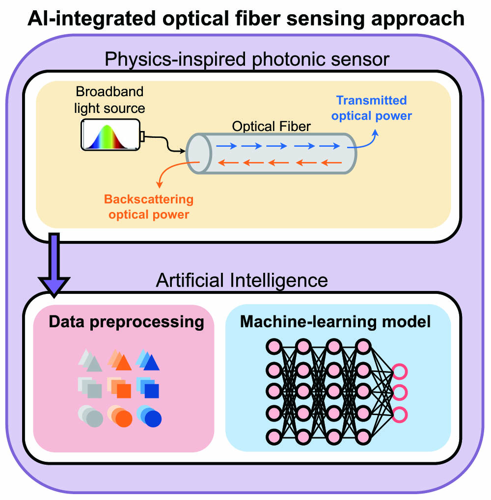
Fig. 1. AI-integrated optical fiber sensing approach as a result of the combination of a photonics sensor and machine learning.
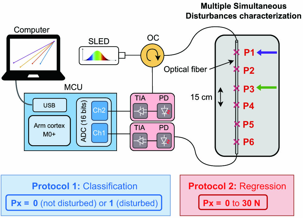
Fig. 2. Experimental setup of the multiple simultaneous disturbances characterization for two protocols.
Fig. 3. FFNN model for both protocols of system’s characterization.
Fig. 4. Smart environment protocol. (a) Smart environment setup: entrance carpet (L1), chair (L2), bathroom handrail (L3), bedroom carpet (L4), bed (L5), and desktop (L6). (b) FFNN model for the smart environment protocol.
Fig. 5. Transmitted and reflected optical powers under three conditions in Protocol 1: (a) single-point perturbation, (b) two-point perturbation, and (c) three-point perturbation.
Fig. 6. Confusion matrices of each label for single and multiple perturbation detection using the FFNN model.
Fig. 7. Results of the force regression for each point (no weight was applied on P6).
Fig. 8. Temporal analysis of real and predicted forces applied on each position.
Fig. 9. Results of transmitted and reflected optical power using the TRA setup for place identification in the smart environment.
Fig. 10. Metrics of the FFNN model with 70 epochs for the identification of the accessed places in the smart environment: (a) loss and (b) accuracy.
Fig. 11. Results of the classification of new data using the designed FFNN model for three different conditions: (a) two persons at home, (b) one person at home, and (c) no person at home.
|
Table 1. Combination of the Multiple Simultaneous Disturbances in Protocol 1 (Disturbance Classification)
|
Table 2. Combination of Different and Simultaneous Weights in Protocol 2 (Force Regression in Newtons)
|
Table 3. Comparison of Outcomes Using Different Machine Learning Algorithms to Classify Events in Distributed Sensing

Set citation alerts for the article
Please enter your email address
© Copyright 2018-2021 | Chinese Laser Press. All Rights Reserved 沪ICP备15018463号-20