
Wei Yin, Yuxuan Che, Xinsheng Li, Mingyu Li, Yan Hu, Shijie Feng, Edmund Y. Lam, Qian Chen, Chao Zuo. Physics-informed deep learning for fringe pattern analysis[J]. Opto-Electronic Advances, 2024, 7(1): 230034
- Opto-Electronic Advances
- Vol. 7, Issue 1, 230034 (2024)
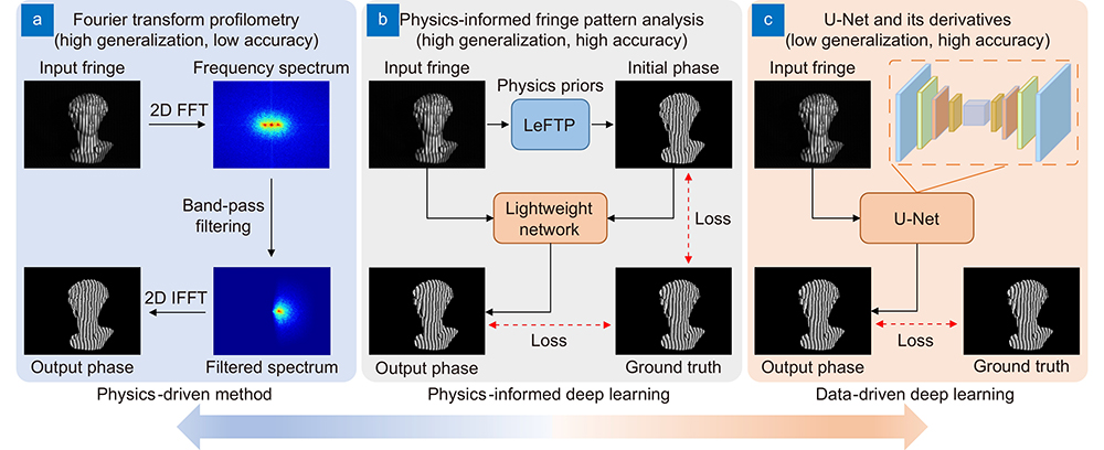
Fig. 1. Diagrams of the physics-driven method, physics-informed deep learning approach, and data-driven deep learning approach for fringe pattern analysis.
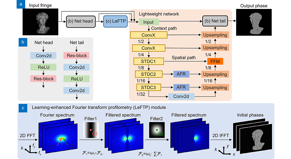
Fig. 2. Overview of the proposed PI-FPA. (a ) PI-FPA including a LeFTP module and a lightweight network. (b ) Net head and Net tail. (c ) The phase retrieval process of the LeFTP module.
Fig. 3. Comparative results for single-shot fringe pattern analysis of the David model. (a –e ) The phase retrieval process, wrapped phases, phase errors, and magnified views of the phase errors using FTP, LeFTP, Net head + LeFTP, U-Net, and PI-FPA.
Fig. 4. Comparative fringe analysis results of the industrial part. (a ) The industrial part and the phase errors using FTP, U-Net, and PI-FPA. (b ) The magnified views of the phase errors. (c ) Single-shot 3D imaging results using different methods. (d ) The magnified views of (c). (e ) The line profiles in (d).
Fig. 5. Precision analysis for a ceramic plane and a standard sphere moving along the Z axis. (a ) 3D reconstruction results using PI-FPA at different time points. (b –c ) the error distributions of the sphere and plane. (d –e ) temporal precision analysis results of the plane and sphere over a 1.62 s period using 3-step PS, FTP, U-Net, and PI-FPA. (f –i ) the color-coded 3D reconstruction and the corresponding error distributions of the plane and the standard sphere using different methods at T = 0.81 s.
Fig. 6. Fast 3D measurement results using different fringe pattern analysis methods. (a ) The representative fringe images at different time points and the corresponding color-coded 3D reconstructions results for the rotated workpiece model using 3-step PS, FTP, U-Net, and PI-FPA. (b ) The representative fringe images at different time points and the corresponding color-coded 3D reconstructions results for non-rigid dynamic face using 3-step PS, FTP, U-Net, and PI-FPA. (c ) 360-degree 3D reconstruction of the workpiece model using PI-FPA. (d ) 3D measurement results of non-rigid dynamic face using PI-FPA.
| ||||||||||||||||||||||
Table 1. Quantitative analysis results of the moving plane and sphere for different methods.

Set citation alerts for the article
Please enter your email address
© Copyright 2018-2021 | Chinese Laser Press. All Rights Reserved 沪ICP备15018463号-20