Sub-diffraction dark spot localization microscopy

Chuankang Li; Yuzhu Li; Zhengyi Zhan; Yuhang Li; Xin Liu; Yong Liu; Xiang Hao; Cuifang Kuang; Xu Liu

doi:10.1364/PRJ.429933

Abstract

Single molecular localization microscopy (SMLM) is a useful tool in biological observation with sub-10-nm resolution. However, SMLM is incapable of discerning two molecules within the diffraction-limited region unless with the help of a stochastic on–off switching scheme which yet entails time-consuming processes. Here, we produce a novel kind of focal spot pattern, called sub-diffraction dark spot (SDS), to localize molecules within the sub-diffraction region of interest. In our proposed technique nominated as sub-diffracted dark spot localization microscopy (SDLM), multiple molecules within the diffraction-limited region could be distinguished without the requirement of stochastic fluorescent switches. We have numerically investigated some related impacts of SDLM, such as detection circle diameter, collected photon number, background noise, and SDS size. Simulative localization framework has been implemented on randomly distributed and specifically structured samples. In either two- or three-dimensional case, SDLM is evidenced to have

\sim 2 nm

localization accuracy.

1. INTRODUCTION

Single-molecule localization microscopy (SMLM), such as stochastic optical reconstruction microscopy [1] or photoactivated localization microscopy [2], circumvents the diffraction limit using centroid estimation of sparsely activated and stochastic switching by acquiring multiple single-molecule fluorescence images [3]. However, SMLM requires a large amount of fluorescent switches which are detrimental for long-term observation. Recently, a new technique called MINFLUX [4 –6] was promoted, in which a doughnut-shaped or standing-wave illumination pattern moves over an area in diameter $L$ , and the position of a single fluorophore in the scanning domain is determined by targeted coordinate pattern based on the detected photon count $N$ for distinct doughnut positions. The issue of maximizing the localization precision with the limited photon flux is well addressed by MINFLUX. The localization precision of this process scales as $L / \sqrt{N}$ . As the scan range $L$ can in principle be chosen arbitrarily small, the localization precision could be ultra-high. The same rationale is also applicable to sinusoidal point-scanning or widefield imaging setup [7,8]. However, the above-mentioned methods are based on diffraction-limited Gaussian or doughnut-shaped spot which is incapable of discerning two molecules within the diffraction-limited region unless the stochastic on–off switching scheme is employed which yet entails time-consuming processes.

Here, we produce a novel kind of focal spot pattern, called sub-diffraction dark spot (SDS), and we propose the sub-diffraction dark spot localization microscopy (SDLM) to discriminate molecules of interest within the diffraction-limited region. Physical mechanics, such as stimulated emission depletion [9], saturated absorption competition [10], or charge state depletion [11], might be equally potential to obtain the SDS. The central dip of the SDS features higher light sensitivity compared with that of the conventional dark spot (CDS). The dependency of the Cramér–Rao bound (CRB) of SDLM on factors such as detection circle diameter (or detection length) $L$ , photon number $N$ , and signal-to-background ratio (SBR), is investigated in two- and three-dimensional cases. A numerical localization framework has been implemented on randomly and specifically distributed molecule ambients. The results show that SDLM is advantageous in molecular localization with $\sim 2 nm$ precision. In the perspective of the easy-to-implement configuration, SDLM is believed to hold great promise to facilitate biomedical and physical discoveries.

2. THEORY

In the focal plane of the SDS, an excitation light spot is overlaid with a depletion light spot, both of which are doughnut-shaped featuring a central intensity minimum. In regions with high depletion intensity $I_{dep}$ , the spontaneous decay of fluorophores is largely suppressed. Nonetheless, those fluorophores residing at or close to the central minimum remain to emit freely. To this end, the off-the-center fluorescence is inhibited and the shrinkage of the resulting spot profile bears similarity to the suppression of Gaussian focal volume in stimulated emission depletion microscopy (STED). The higher power density of the depletion beam is employed, the more suppression of dark spot occurs.

Sign up for Photonics Research TOC. Get the latest issue of Photonics Research delivered right to you！Sign up now

We define the inhibition coefficient $η (r)$ as the fraction of fluorescence still detected at position $r$ in the presence of depletion light of intensity $I_{dep} (r)$ . The inhibition coefficient can usually be well approximated by an exponential [12,13]: $η (r) = \exp [- \ln (2) I_{dep} (r) / I_{s}],$ (1) $I_{s} = k_{f} h c / (σ λ),$ (2)where $I_{s}$ stands for the saturation intensity (at which the rate of stimulated emission equals the spontaneous decay), $k_{f}$ is the rate constant of spontaneous fluorescence, $h$ denotes the Planck constant, $c$ is the light velocity, $σ$ denotes the cross section of fluorescence emission, and $λ$ is the depletion wavelength. The point spread function (PSF) of the hollow excitation beam $I_{hexc} (r)$ or depletion beam $I_{dep} (r)$ can be expressed by Eq. (3) [4]: ${PSF}_{hexc / dep} (r) {= A}_{0} 4 e \ln (2) \frac{r^{2}}{{FWHM}^{2}} e^{- 4 \ln (2) \frac{r^{2}}{{FWHM}^{2}}},$ (3)where $A_{0}$ is the peak intensity for the doughnut-shaped beam (the depletion beam or hollow excitation beam), and FWHM is a size-related parameter for the doughnut beam profile. Thus, the effective PSF of the SDS is given by Eq. (4): ${PSF}_{SDS} (r) {= PSF}_{hexc} (r) \cdot η (r) .$ (4)

Due to the exponential behavior in Eq. (1), ${PSF}_{SDS}$ is also a doughnut-shaped profile with a reduced width along the radial direction. Note that this modality can also be suitable for the axial scenario while using the axial dark spot.

Taking 2D localization for illustration, the dark spot is placed in four anticipated positions $r_{i}$ ( $i$ denotes the position number) and the certain fluorescent molecule in position $r_{m}$ to be localized is exposed to four different laser powers $I_{i}$ . To this end, the detector will receive different photon counts $n_{i}$ . Note that $n_{i}$ will contribute to specific spatial probability distribution in each localization period. Based on the photon count distribution we have obtained in each localization cycle, we calculate the reciprocal spatial probability distribution for each position in the region of interest (ROI). According to the maximum likelihood estimator principle, we select the maximal probability value of the spatial position as the molecule position which is most likely to be located. For 3D ambient, two additional placements in the axial direction are necessary to identify the $Z$ -axis position of the molecule.

After acquiring different photon numbers $n_{i}$ , the total acquired photon number is $N = n_{0} + n_{1} + \dots + n_{k - 1}$ with $i \in [0, \dots, k - 1]$ , where $k$ denotes the total position number of the beam displacements. Note that each acquired photon number $n_{i}$ follows the Poisson statistic with a mean $μ_{i}$ . We nominate the spatial success probability distribution $p_{i}^{(0)}$ when the hollow beam center is in the $i$ -th position, regardless of the contribution of the background and dark counts: $p_{i}^{(0)} = \frac{μ_{i}}{\sum_{j = 0}^{k - 1} μ_{j}} with j \in [0, \dots, k - 1] .$ (5)

However, the influence of background is inevitable for realistic world imaging. It is assumed that the background contribution also follows the Poisson statistic with a mean $β_{i}$ for each signal detection. The signal-to-background ratio $SBR = \sum_{i = 0}^{k - 1} μ_{i} / \sum_{i = 0}^{k - 1} β_{i}$ is defined. Thus, in consideration of background contribution, $p_{i}$ can be written as [4]

$p_{i} = \frac{SBR}{SBR + 1} p_{i}^{(0)} + \frac{1}{k (SBR + 1)} .$ (6)

Obviously, when the SBR becomes infinity, $p_{i}$ equals $p_{i}^{(0)}$ . In each positon $r_{i}$ , different signal strength $μ_{i}$ is acquired, expressed as follows using Eqs. (1)–(4): $μ_{i} {= PSF}_{hexc} ({\bar{r}}_{m} - {\bar{r}}_{i}) \cdot η (r) {= PSF}_{hexc} ({\bar{r}}_{m} {- \bar{r}}_{i}) \exp [- \ln (2) \frac{{PSF}_{dep} ({\bar{r}}_{m} - {\bar{r}}_{i})}{k_{f} h c / (σ λ)}] .$ (7)

Since each acquisition of the photon count $n_{i}$ is independent, the photon count distribution $L (\bar{p}, \bar{n})$ obeys the polynomial equation as follows: $L (\bar{p}, \bar{n}) = \frac{N!}{Π_{i = 0}^{k - 1} n_{k}!} Π_{i = 0}^{k - 1} p_{i}^{n_{i}} .$ (8)

The Fisher information $F_{\bar{p}}$ is introduced to quantitatively reflect the information of the position of fluorescent molecules carried by the measured photon distribution: $F_{\bar{p}} = E [- \frac{\partial^{2}}{\partial p_{i} \partial p_{j}} \ln L (\bar{p}, \bar{n})] with i, j \in [0, \dots, k - 1] .$ (9)

Operating with Eq. (8), the Fisher information matrix for $\bar{p}$ is obtained: $F_{\bar{p}} = N (\frac{1}{p_{k - 1}} + δ_{i j} \frac{1}{p_{i}}),$ (10)where $δ_{i j}$ is the Kronecker delta function. We use the Jacobian matrix to transform $F_{\bar{p}}$ to the $\bar{r}$ -space Fisher information $F_{\bar{r}}$ , which corresponds the photon distribution probability $L (\bar{p}, \bar{n})$ to the fluorescent molecule position ${\bar{r}}_{m} = {[r_{1}, \dots, r_{d}]}^{T}$ in $d$ -dimensional space: $F_{\bar{r}} = N \sum_{i = 0}^{k - 1} \frac{1}{p_{i}} (\begin{matrix} {(\frac{\partial p_{i}}{\partial r_{i}})}^{2} & \dots & \frac{\partial p_{i}}{\partial r_{1}} \frac{\partial p_{i}}{\partial r_{d}} \\ ⋮ & ⏧ & ⋮ \\ \frac{\partial p_{i}}{\partial r_{d}} \frac{\partial p_{i}}{\partial r_{1}} & \dots & {(\frac{\partial p_{i}}{\partial r_{d}})}^{2} \end{matrix}) .$ (11)

In our work, the arithmetic mean $σ_{CRB} = \sqrt{t r (F_{\bar{r}}^{- 1}) / d}$ is defined to calculate the localization precision of our method. The CRB provides a lower bound for the variance of any unbiased estimator [14 –16]. Smaller $σ_{CRB}$ leads to smaller parameter estimation error of the localization method; thereby the higher accuracy of the estimation can be obtained. As for lateral condition in the lateral plane ( $d = 2$ ), the $σ_{CRB}$ can be expressed as follows: $σ_{CRB_x y} = \sqrt{\frac{1}{2 N} \frac{\sum_{i = 0}^{k - 1} \frac{1}{p_{i}} [{(\frac{\partial p_{i}}{\partial x})}^{2} + {(\frac{\partial p_{i}}{\partial y})}^{2}]}{[\sum_{i = 0}^{k - 1} \frac{1}{p_{i}} {(\frac{\partial p_{i}}{\partial x})}^{2}] [\sum_{i = 0}^{k - 1} \frac{1}{p_{i}} {(\frac{\partial p_{i}}{\partial y})}^{2}] - {[\sum_{i = 0}^{k - 1} \frac{1}{p_{i}} \frac{\partial p_{i}}{\partial x} \frac{\partial p_{i}}{\partial y}]}^{2}}} .$ (12)

As for axial condition ( $d = 1$ for the $Z$ direction), the $σ_{CRB}$ can be expressed as follows: $σ_{CRB_z} = \frac{1}{N \sum_{i = 0}^{k - 1} \frac{1}{p_{i}} {(\frac{\partial p_{i}}{\partial z})}^{2}} .$ (13)

3. SIMULATION AND DISCUSSION

The CDS and SDS are shown in Figs. 1(a) and 1(b), respectively. The intensity distributions of CDS and SDS are $I_{hexc}$ and $I_{SDS}$ , respectively. In Fig. 1(a), the normalized crest intensity ratio of the lateral and axial dark spot is 1:0.6. It is seen from Fig. 1(b) that the SDS is greatly suppressed compared with the CDS. In the inset top-left graph of Fig. 1(d), two concepts concerning the dark spots are presented: the FWHM and outer FWHM (oFWHM). Shown in Fig. 1(d), the numerical results indicate that the lateral FWHM and lateral oFWHM values of 3D $I_{SDS}$ are greatly squeezed by a factor of 4.8 and 4.5, respectively. The squeezed dip of $I_{SDS}$ yields a conspicuous gradient featuring high light-intensity sensitivity and is helpful to molecular localization. Furthermore, the suppressed peripheral part of the SDS contributes to discerning multiple molecules in the diffraction-limited ROI without the need of stochastic fluorescent switches. With the increase of depletion beam intensity, the value of oFWHM could be further decreased from Eqs. (1)–(4).

$(a) Lateral and axial PSFs of 3D diffraction-limited dark spot of hollow excitation beam (Ihexc). (b) The lateral and axial PSFs of 3D sub-diffraction dark spot (SDS). (c) Numerical imaging comparison of Iexc,ISTED, and ISDS. The simulative areas are all 2 μm×2 μm with 10-nm pixel. (d) Normalized intensity curves of hollow depletion beam (Idep), ISTED, and ISDS. (e) The MTF analysis of Iexc,Ihexc, ISTED, and ISDS. The spatial frequency values are normalized by 2π NA/λ. NA: 1.4;λ: 532 nm; Iexc: 10 kW/cm2; Ihexc: 10 kW/cm2; Idep: 5 MW/cm2. (f) The working principle comparison between MINFLUX (upper row) and SDLM (lower row). The depletion beam intensities of 50–100 MW/cm2 are applied. wf, wide field. (g) The schematic of the optical setup of SDLM. The four deflections of the excitation pattern in specific positions are called excitation beam patterning (EBP). OL, objective lens. Scale bars in all: 200 nm.$

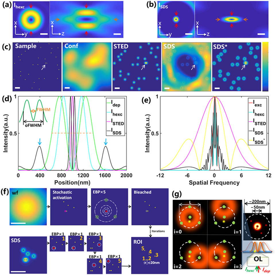
Figure 1.(a) Lateral and axial PSFs of 3D diffraction-limited dark spot of hollow excitation beam ( $I_{hexc}$ ). (b) The lateral and axial PSFs of 3D sub-diffraction dark spot (SDS). (c) Numerical imaging comparison of $I_{exc}, I_{STED}$ , and $I_{SDS}$ . The simulative areas are all $2 μm \times 2 μm$ with 10-nm pixel. (d) Normalized intensity curves of hollow depletion beam ( $I_{dep}$ ), $I_{STED}$ , and $I_{SDS}$ . (e) The MTF analysis of $I_{exc}, I_{hexc}, I_{STED}$ , and $I_{SDS}$ . The spatial frequency values are normalized by $2 π NA / λ$ . $N A : 1.4; λ : 532 nm$ ; $I_{exc} : 10 {kW / cm}^{2}$ ; $I_{hexc} : 10 {kW / cm}^{2}$ ; $I_{dep} : 5 {MW / cm}^{2}$ . (f) The working principle comparison between MINFLUX (upper row) and SDLM (lower row). The depletion beam intensities of $50 - 100 {MW / cm}^{2}$ are applied. wf, wide field. (g) The schematic of the optical setup of SDLM. The four deflections of the excitation pattern in specific positions are called excitation beam patterning (EBP). OL, objective lens. Scale bars in all: 200 nm.

From Fig. 1(c), the imaging comparison of different focal spots is simulated. Although the FWHM of the resulting SDS is greatly squeezed, sidelobes occur denoted by the blue arrows shown in Fig. 1(d), which are derived from the insufficiently depleted fluorescence in the outermost part of the focal spots. These sidelobes degrade the image quality and localization effect, which should be avoided for high-contrast imaging. The sidelobes could be removed by loading doughnut patterns with higher topological charges via devices such as spatial light modulators. The modulated transfer function (MTF) is also analyzed shown in Fig. 1(e). The cutoff frequency from the highest to the lowest is as follows: $I_{SDS *}, I_{STED}, I_{SDS}, I_{hexc}, I_{exc}$ . It is clearly seen that $I_{SDS *}$ has a larger spatial frequency component than $I_{STED}$ . SDS* denotes the SDS result with sidelobes removed [10]. If not otherwise specified, the sidelobes of the SDS in the following discussion are considered to be removed. It is also evidenced from the white arrows in Fig. 1(c) where the two molecules, which are indistinguishable by STED, could be resolved by the SDS. Figures 1(f) and 1(g) show the working principle of SDLM.

In Fig. 1(f), five features are all in the diffraction-limited region. For MINFLUX, the molecular localization iteration is as follows: stochastic activation, excitation beam pattern (EBP) sequences, and bleaching. For SDLM, a point-wise scanning image is first obtained for coarse localization. It is found that there is more than one molecule in the left-bottom corner. Hence, the depletion beam intensity is increased to $100 {MW / cm}^{2}$ so that the far detailed molecule spatial information is further extracted. Only one EBP sequence is subsequently applied to achieve nanometer-scale localization. As for the remnant molecules, lower depletion intensity, like $50 {MW / cm}^{2}$ , is sufficient for molecular localization. For a nanometer-scale localization of each molecule in MINFLUX, $\sim 1 s$ is required. For SDLM, since the activation process is not needed and the times of EBP sequences are reduced, even less time is estimated.

The dependence of depletion beam intensity $I_{dep}$ on the resulting three-dimensional SDS profile is researched in the lateral and axial planes. From Figs. 2(a) and 2(b), the FWHM values decrease with the increase of depletion illumination power from 100 nm to 44 nm. Likewise, the oFWHM values can be lower than 100 nm in the case that $9 {MW / cm}^{2}$ or larger $I_{dep}$ is applied. In Figs. 2(c) and 2(d), the dependence of $I_{dep}$ on the resulting SDS profile in the axial direction is investigated. The FWHM values decrease with the increase of depletion illumination power from 260 nm to 100 nm. In our scheme, the lateral and axial oFWHM values are accommodated with $\sim 50 nm$ and $\sim 150 nm$ , respectively, when $50 {MW / cm}^{2}$ is employed.

Figure 2.PSFs of $I_{SDS}$ with different $I_{dep}$ for 3D SDS. (a) The PSFs of $I_{SDS}$ for lateral dark spots in the lateral plane ( $I_{dep} = 1 - 7 {MW / cm}^{2}$ ). (b) The dependence of the FWHM and oFWHM on $I_{dep}$ for lateral dark spots ( $I_{dep} = 1 - 9 {MW / cm}^{2}$ ). (c) The PSFs of $I_{SDS}$ for axial dark spots in the axial plane ( $I_{dep} = 1 - 7 {MW / cm}^{2}$ ). (d) The dependence of the FWHM and oFWHM on $I_{dep}$ for axial dark spots ( $I_{dep} = 1 - 9 {MW / cm}^{2}$ ).

4. RESULTS

From the above-mentioned simulations, we can obtain an effective doughnut pattern, which has both smaller oFWHM and FWHM values, approximately one fourth of the CDS. Compared with the CDS, applying this sub-diffracted dark spot to nanometer localization will confine the excited fluorescent emitters to a smaller region so that discerning two molecules within the diffraction limit without the help of stochastic on–off switching becomes possible. The lateral localization work of SDLM is conducted; $L$ is the diameter of the detection circle which corresponds to four SDS placements and $N$ is the detected photon number for localization. Considering the real-world circumstance, background contribution is added in our simulation, referring to Eq. (6). From Figs. 3(a) and 3(b), when $SBR = 30$ and $N = 50$ , the CRB values in the lateral localization for the origin of the detection circle are shown. It is seen that with the decrease of $L$ , the localization precision is enhanced from 1.2 nm to 0.2 nm. With the increase of $N$ , the precision is also enhanced. While the detection circle diameter is determined, e.g., $L = 20 nm$ , the CRB of each position in the whole detection region is investigated. The color mapping in Fig. 3(c) indicates that in the center of the clover-shaped region, the highest precision is achieved (about 1.19 nm). The dashed circle presents the boundary of localization precision of 2.23 nm. It is worth noting that three abnormal points are observed in positions corresponding to 60, 180, 300 deg, respectively. It might be caused by insufficient covering of four beam placements.

Figure 3.(a) CRB values in the lateral localization for the origin of the lateral detection circle when $L_{x y} = 4 - 20 nm$ . (b) The statistics histogram of CRB for the origin of the lateral detection circle when $N = 50 - 350$ . The inset top-right graph shows the beam deflections in four specific positions in the $X Y$ plane. (c) CRB color mapping of SDLM via lateral localization for the whole region of the detection circle in the $X Y$ plane when $L_{x y} = 20 nm$ , $N = 50$ , and $SBR = 30$ . (d) The CRB values in the axial localization for the origin of the axial detection when $L_{z} = 4 - 20 nm$ . (e) The statistics histogram of CRB for the origin of the axial detection when $N = 50 - 35$ . The inset top-right graph shows the beam deflections in three specific positions in the $Z$ -axis direction. (f) CRB curves of SDLM via $Z$ -axis localization along the whole axial detection length when $L_{z} = 20 nm$ , $N = 50 - 350$ , and $SBR = 30$ . $I_{dep} = 30 {MW / cm}^{2}$ is applied for the above-mentioned SDLM. (g), (h) The influence of background noise on the lateral and axial CRB values when $N = 50$ .

Similarly, three beam placements (positive defocus, in-focus, negative defocus) are applied to obtain axial localization precision. For the axial origin, Figs. 3(d) and 3(e) present the dependence of the CRB on $L$ and $N$ . It is found that compared with the lateral scenario, the axial precision is even higher (ranging from 0.6 to 0.1 nm). Evidenced by Fig. 2, in the lateral direction, it presents a much sharper fluorescence intensity gradient than that in the axial direction. Hence, with the increase of detection circle diameter (or detection length) $L$ , the lateral localization precision presents a much more pronounced trend than the axial one. That is the reason why the CRB estimations for the axial and the lateral directions are split up. In Fig. 3(f), when $L = 20 nm$ and $N = 50$ , the CRB values for each position along the axial direction are simulated. In the axial origin, 0.5-nm localization precision is achieved. Gradually apart from the center, the CRB increases to 3 nm. The aforementioned results are all included with noise factor ( $SBR = 30$ ). It is concluded that in the detection range of 20 nm, sub-3-nm localization precision is achieved in the 3D case.

Background noise contributes to the resulting localization precision to some extent, as shown by Figs. 3(g) and 3(h). In the lateral condition, when $L = 20 nm$ and $N = 50$ , with the increase of SBR from 3 to 100, the localization precision is enhanced from 1.6 nm to 1.2 nm with a 25% improvement. Similarly, as for the axial condition, CRB values decrease from 1 nm to 0.6 nm with a 40% improvement. In the future, the underlying background noise formula is expected to be further investigated in order to evaluate our method in a realistic manner. For instance, in our work, the SBR is independent of beam displacement $r_{i}$ and is considered as a constant. In another noise model, $SBR (r_{i})$ could be related with the position $r_{i}$ , especially for $SBR (r_{0})$ which is related with the origin position $r_{0}$ .

In order to further investigate the relationship between SDS size and localization precision via SDLM, we select four kinds of SDS for localization analysis: SDLM with different oFWHM values, corresponding to $\sim 50 nm$ , $\sim 100 nm$ , $\sim 150 nm$ , and $\sim 200 nm$ , respectively. From Figs. 4(a) and 4(b), while $L = 10 - 20 nm$ , $N = 50$ , and $SBR = 30$ , those dark spot patterns present a slight rise in CRB which is lower than 1 nm in either the lateral or axial direction. However, when $L$ is larger than 20 nm, SDLM with $\sim 50 nm$ shows pronounced growth and its lateral localization precision becomes especially worse. As we have mentioned before, it is due to the insufficient covering of four beam placements of small size SDS. Thus, a decreased size of SDS is inhibited by a maximum value of detection circle diameter, e.g., for $\sim 50 nm$ SDS, $L$ should not be larger than 20 nm.

Figure 4.(a) Lateral CRB comparison (in the origin of the detection circle) between different sizes of SDS: oFWHM of $\sim 50 nm$ , $\sim 100 nm$ , $\sim 150 nm$ , and $\sim 200 nm$ , respectively, while different depletion powers are applied when $L = 10 - 40 nm$ and $N = 50$ . (b) The axial CRB comparison between different sizes of SDS when $L = 10 - 40 nm$ and $N = 50$ . (c) Root mean square error (RMSE) comparison between SDLM methods with different oFWHM values based on the 11 evenly distributed test points on the diagonal of the cylinder in the 3D case. (d) Localization result of SDLM on 3D randomly distributed molecule concentration ambients. The photon number is 200 used in those simulations. Each $X Y$ plane contains 30 random molecules. Five $X Y$ planes and five $X Z$ planes are selected for observation. It is clearly seen that SDLM can well restore the distribution characteristics of scattered points. (e), (f) RMSE quantitative analysis of molecules either on the lateral plane or on the axial plane.

However, without the implementation of stochastic fluorescent switching, large size SDS may fail to localize multiple features in the sub-diffraction region. In order to evaluate the 3D localization ability of SDLM with different oFWHM values in high molecular density ambient, a verification experiment is conducted accordingly. Molecules with equidistance distribution of 50 nm along the diagonal of the cylinder are characterized using $\sim 50 nm$ and $\sim 200 nm$ SDS. The root mean square error (RMSE) comparison is shown by Fig. 4(c). The error between the estimated position and the actual position could be measured by the RMSE. It is found that SDLM with $\sim 200 nm$ oFWHM shows high average mean and standard deviation values. In contrast, SDLM with $\sim 50 nm$ oFWHM presents sub-2-nm localization precision and the best RMSE is lower than 1 nm. In practical experiment, there should be a careful balance between $L$ , $N$ , SBR, and SDS size in order for the highest localization precision.

Here, we further expand the experiment to more complex conditions, using a randomly distributed map and a specifically shaped map, to test the localization effect of SDLM by adding Poisson noise to match the real experimental ambient. These two models have certain universality and are suitable for simulating the imaging process of some biological structures. We randomly generate some emitters in the whole field of view shown in Fig. 4(d). RMSE results of SDLM with $\sim 50 nm$ oFWHM are shown by Figs. 4(e) and 4(f). The features are dispersed three-dimensionally and the simulation ambient in the $X Y$ plane is several times as dense as the ambient in the $X Z$ plane. SDLM with $\sim 50 nm$ and $\sim 200 nm$ oFWHM can both obtain good localization results in sparse solution of $X Z$ plane images. It also suggests that SDLM could achieve high axial localization precision in sparsely packed fluorophore solution from Fig. 4(e). In the densely packed $X Y$ plane image, $\sim 50 nm$ SDS can almost map out the true information of the sample and the average RMSE of those planes is 1.44 nm seen from Fig. 4(f). In contrast, most of the molecules are not restored using $\sim 200 nm$ SDS.

If we change the map to a specific letter structure, the difference of localization results between the $\sim 50 nm$ SDS and the $\sim 200 nm$ SDS can also be well presented in Fig. 5(a). Figures 5(b) and 5(c) show the RMSE quantitative analysis of molecular localization. The average RMSEs of lateral planes and axial planes are 1.66 nm and 1.51 nm, respectively. We choose the lattice of letters “A” as the fluorescent molecules and the letter “A” is placed in different layers. In order to observe the effect in the $X Y$ plane, five planes corresponding to different $Z$ -axis values (with 200-nm spacing) are compared. Five $X Z$ planes are also discussed with 500-nm separation to estimate the lateral localization ability of SDLM. Although not all the features of the letter “A” are included by SDLM, the outline can be roughly seen. Due to the influence of background noise, the position inaccuracy is increased. The photon budget is set to be 200. The detection circle diameter in the $X Y$ plane and detection length in the $Z$ axis are both 20 nm. By contrast, the $\sim 200 nm$ SDS fails to discriminate most of the molecules.

Figure 5.(a) Localization results of SDLM on the 3D letter “A” shaped map. The photon number is 200 in those simulations while $L = 20 nm$ . (b), (c) RMSE quantitative analysis of molecules either on the lateral plane or on the axial plane.

5. CONCLUSION AND OUTLOOK

This paper presents the principle of SDLM, as well as the simulation work of nanoscale localization applications. It is worth noting that SDLM is a conspicuous combination of SMLM and STED. It is concluded that dark-spot-based localization nanoscopy, such as MINFLUX and SDLM, has the advantage of high localization precision with low photon flux. Note that MINFLUX and SDLM both require for the prerequisite of single molecule excitation during each localization iteration. However, in the aspect of molecular on–off principle, SDLM is completely different from MINFLUX. As for MINFLUX, only one molecule is activated and others remain silent so that the localization sequence could be ensured, while, by virtue of the stimulated emission depletion effect in SDLM, the only molecule of interest in the doughnut center is registered for primary coarse localization, leaving those off-the-center features residing at the ground state.

We have emphasized the exceptional performance of SDLM, but some issues have to be clarified. The fluorescent nanoprobes with special excitation-emission spectrum compatible for stimulated emission depletion will be highly desirable. SDLM is especially compatible for the labeling system in which the molecules are adjacent with $\sim 50 nm$ spacing. In order to characterize even higher molecule density target (e.g., higher than $400 molecules / {μm}^{2}$ ), the reciprocal depletion power has to be further increased which is detrimental to organic dyes in biological utilizations. Inorganic, nonbleaching fluorescent probes, such as quantum dots and fluorescent nanodiamonds [10], will be applicable to biomedical circumstances with high dye concentration. In addition, upconversion nanoparticles (UCNPs) are also potential for SDLM in order to reduce the applied depletion power since the saturation intensity of UCNPs features 2 orders of magnitude lower than that of conventional fluorescent probes [17].

As we know, a nonperfect intensity zero of a doughnut plays an important role in the localization result. Also, the aberration puts an upper limit to the applicable localization accuracy of SDLM. In the future, more quantified study is expected to be carried out considering more realistic factors. In our further study, experimental work will be conducted and the attainable resolution of SDLM could be evaluated by extensive approaches, such as Fourier ring correlation [18]. As one of the advanced molecular localization mechanisms, SDLM is believed to hold great potential in biological and physical applications and to become another powerful tool for the study of the micro world through the follow-up research.

References

[1] M. J. Rust, M. Bates, X. Zhuang. Sub-diffraction-limit imaging by stochastic optical reconstruction microscopy (STORM). Nat. Methods, 3, 793-795(2006).

[2] E. Betzig, G. H. Patterson, R. Sougrat, O. W. Lindwasser, S. Olenych, J. S. Bonifacino, M. W. Davidson, J. Lippincott-Schwartz, H. F. Hess. Imaging intracellular fluorescent proteins at nanometer resolution. Science, 313, 1642-1645(2006).

[3] C. Li, C. Kuang, X. Liu. Prospects for fluorescence nanoscopy. ACS Nano, 12, 4081-4085(2018).

[4] F. Balzarotti, Y. Eilers, K. C. Gwosch, A. H. Gynna, V. Westphal, F. D. Stefani, J. Elf, S. W. Hell. Nanometer resolution imaging and tracking of fluorescent molecules with minimal photon fluxes. Science, 355, 606-612(2017).

[5] Y. Eilers, H. Ta, K. C. Gwosch, F. Balzarotti, S. W. Hell. MINFLUX monitors rapid molecular jumps with superior spatiotemporal resolution. Proc. Natl. Acad. Sci. USA, 115, 6117-6122(2018).

[6] K. C. Gwosch, J. K. Pape, F. Balzarotti, P. Hoess, J. Ellenberg, J. Ries, S. W. Hell. MINFLUX nanoscopy delivers 3D multicolor nanometer resolution in cells. Nat. Methods, 17, 217-227(2020).

[7] L. Gu, Y. Li, S. Zhang, Y. Xue, W. Li, D. Li, T. Xu, W. Ji. Molecular resolution imaging by repetitive optical selective exposure. Nat. Methods, 16, 1114-1120(2019).

[8] J. Cnossen, T. Hinsdale, R. O. Thorsen, M. Siemons, F. Schueder, R. Jungmann, C. S. Smith, B. Rieger, S. Stallinga. Localization microscopy at doubled precision with patterned illumination. Nat. Methods, 17, 59-63(2020).

[9] S. W. Hell, J. Wichmann. Breaking the diffraction resolution limit by stimulated emission: stimulated-emission-depletion fluorescence microscopy. Opt. Lett., 19, 780-782(1994).

[10] C. K. Li, Y. H. Li, Y. B. Han, Z. M. Zhang, Y. Z. Li, W. S. Wang, X. Hao, C. F. Kuang, X. Liu. Pulsed saturated absorption competition microscopy on nonbleaching nanoparticles. ACS Photonics, 7, 1788-1798(2020).

[11] X. D. Chen, C. L. Zou, Z. J. Gong, C. H. Dong, G. C. Guo, F. W. Sun. Subdiffraction optical manipulation of the charge state of nitrogen vacancy center in diamond. Light Sci. Appl., 4, e230(2015).

[12] B. Harke, J. Keller, C. K. Ullal, V. Westphal, A. Schoenle, S. W. Hell. Resolution scaling in STED microscopy. Opt. Express, 16, 4154-4162(2008).

[13] M. Leutenegger, C. Eggeling, S. W. Hell. Analytical description of STED microscopy performance. Opt. Express, 18, 26417-26429(2010).

[14] R. J. Ober, S. Ram, E. S. Ward. Localization accuracy in single-molecule microscopy. Biophys. J., 86, 1185-1200(2004).

[15] J. Chao, E. S. Ward, R. J. Ober. Fisher information theory for parameter estimation in single molecule microscopy: tutorial. J. Opt. Soc. Am. A, 33, B36-B57(2016).

[16] P. Zeiger, L. Bodner, L. Velas, G. J. Schuetz, A. Jesacher. Defocused imaging exploits supercritical-angle fluorescence emission for precise axial single molecule localization microscopy. Biomed. Opt. Express, 11, 775-790(2020).

[17] Q. Zhan, H. Liu, B. Wang, Q. Wu, R. Pu, C. Zhou, B. Huang, X. Peng, H. Agren, S. He. Achieving high-efficiency emission depletion nanoscopy by employing cross relaxation in upconversion nanoparticles. Nat. Commun., 8, 1058(2017).

[18] S. Koho, G. Tortarolo, M. Castello, T. Deguchi, A. Diaspro, G. Vicidomini. Fourier ring correlation simplifies image restoration in fluorescence microscopy. Nat. Commun., 10, 3103(2019).