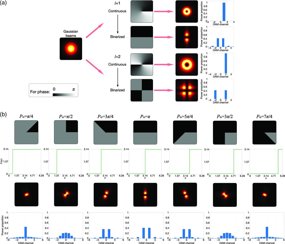
Fig. 1. Binarizing continuous azimuthal phases into 0-π azimuthal binary phases. (a) The binarization of continuous azimuthal phases with one and two nodal lines (the first- and second-order SPPs) under the threshold Pth=π. The binarized phase can produce symmetric OAM components with respect to l=0 mode, compared with the corresponding continuous azimuthal phases. (b) The 0-π phase binarized under various binarization threshold Pth as π/4, π/2, 3π/4, π, 5π/4, 3π/2, and 7π/4, respectively. First to fourth lines in panel (b): the phase distribution, the phase versus the azimuthal angle φ, the simulated far-field diffraction pattern, and the corresponding calculated OAM spectrum.

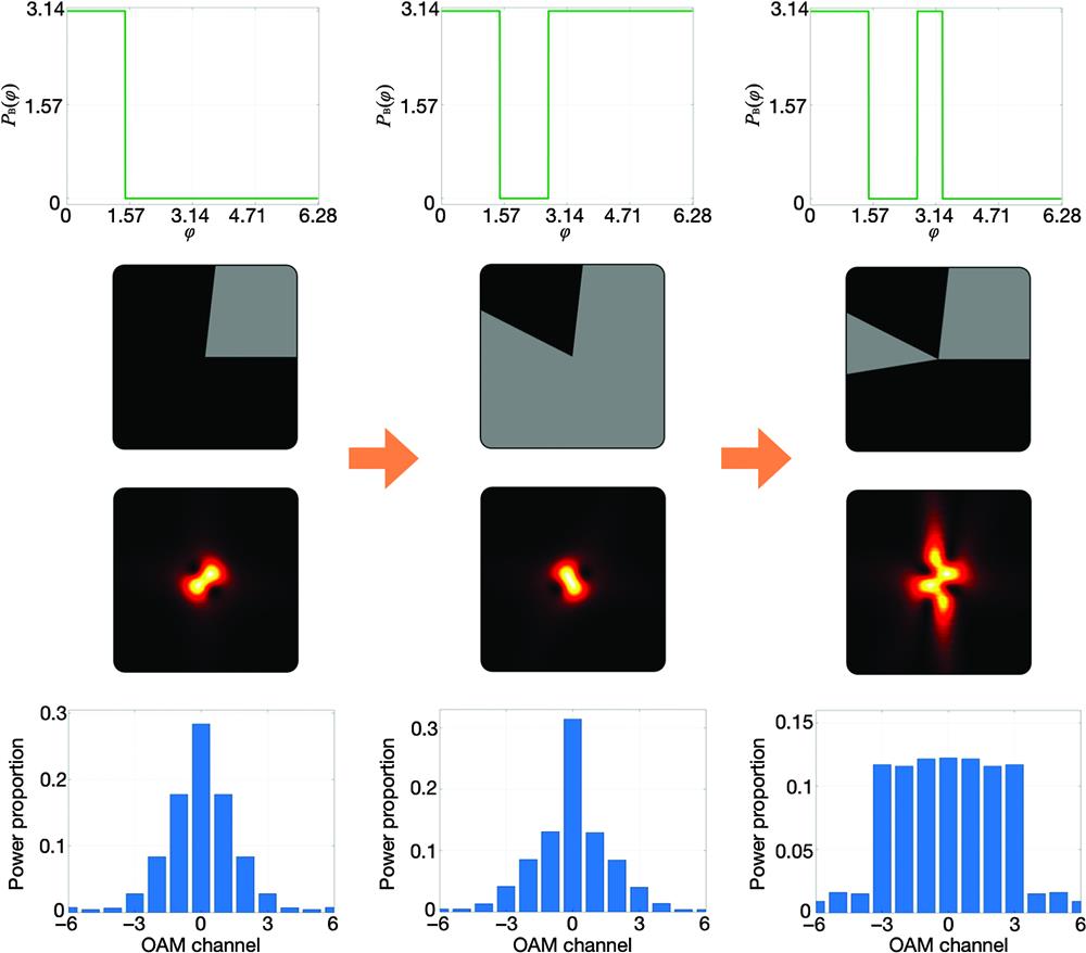
Fig. 2. The evolution of the obtained OAM spectra with respect to azimuthal transition points. Four transition points as φ0=0, φ1=1.4564, φ2=2.6703, and φ3=3.3015 are introduced orderly in the azimuthal section [0,2π) as an example to demonstrate OAM spectrum variation. From top to bottom are the azimuthal transition points, the corresponding azimuthal binary phases, far-field diffraction patterns, and OAM spectra. Obviously, the number and value of transition points determine the final obtained OAM spectra.

Fig. 3. OAM comb manipulation with various OAM mode intervals. From left to right are azimuthal transition points, the corresponding binary phases, far-field diffractions, and OAM combs, respectively. All the OAM combs in (a), (b), and (c) consist of nine OAM components, but their OAM mode intervals are different as 1, 2, and 3, respectively. The interval difference results by scaling the azimuthal phase φ.

Fig. 4. Experimentally generated OAM combs. (a) Experimental results of an OAM comb consisting of 64 OAM states ranging from −63 to +63 with the OAM mode interval Δl=2. (b) Experimental results of an OAM comb consisting of 64 OAM states ranging from −62 to +62 with the OAM mode interval Δl=4. In both of the cases the OAM spectra are measured through anti-SPP based OAM back-conversion.