The resonant enhancement of both optical and mechanical response in a cavity optomechanical system [1,2] has enabled precision sensors [3] of displacement [4,5], force [6], mass [7], acceleration [8,9], ultrasound [10], and magnetic fields [11–17]. Cavity optomechanical magnetometers are particularly attractive, promising state-of-the-art sensitivity without the need for cryogenics, with only microwatt power consumption [11–13,15–17], and with silicon chip-based fabrication offering scalability [16]. For instance, cavity optomechanical magnetometers working in the megahertz frequency range have been demonstrated by using a magnetostrictive material Terfenol-D, either manually deposited onto a microcavity [11,12,15] with a reported peak sensitivity of 200pT/Hz [12], or sputter coated onto the microcavity with a reported peak sensitivity of 585pT/Hz [16]. Efforts have also been made to improve the sensitivity in the hertz-to-kilohertz frequency range, which is relevant to many applications. The nonlinearity inherent in magnetostrictive materials has been used to mix the low frequency signals up to high frequency [12]; a peak sensitivity of 131pT/Hz has been reported in the 100 kHz range using a centimeter-sized CaF2 cavity with a cylinder of Terfenol-D crystal embedded inside [13]; and polymer coated microcavities have been combined with millimeter-sized magnets to provide a sensitivity of 880pT/Hz at 200 Hz [17]. Resonant magnon assisted optomechanical magnetometers have recently been realized, achieving a sensitivity of 103pT/Hz in the gigahertz (GHz) frequency range [18], while torque magnetometers have also been demonstrated using nanomechanical systems for magnetization measurement [19,20]. With all of this recent progress, however, the sensitivity of the best optomechanical magnetometers remains around an order of magnitude inferior to similarly sized cryogenic magnetometers [21–23].

This paper focuses on optimizing the sensitivity of magnetostrictive optomechanical magnetometers. We find that the sensitivity depends critically on the shape of the support that suspends the magnetometer above the silicon chip. This support both constrains the magnetostriction-induced mechanical motion and provides an avenue for thermal fluctuations to enter the system. By engineering its structure to increase both its compliance and the mechanical quality factor of the device, we demonstrate around an order of magnitude improvement in sensitivity compared to previous works, to 26pT/Hz. This is comparable to the similarly sized cryogenic magnetometers [21–23].

The magnetic response as a function of magnetic field frequency is found to show two significantly different behaviors: a relatively smooth response modulated by the mechanical resonances of the structure and a response that exhibits dramatic variations as a function of frequency, with these variations occurring under the envelope of the mechanical resonances. We refer to these two behaviors as Type I and Type II, respectively. The magnetic response of the Type II devices is observed to be highly sensitive to direct current (DC) magnetic fields. We find this behavior is consistent with interference of acoustic waves produced at multiple grain boundaries in a polycrystalline Terfenol-D particle. We therefore infer that the Type I and II responses arise when the particle is mono- and polycrystalline, respectively. Our devices, therefore, provide a method to characterize the Terfenol-D crystal structure, a measurement which is generally challenging at the level of a single grain.

The magnetometers show an ultrabroadband response. The working frequency ranges for both Type I and Type II magnetometers are more than 130 MHz, limited by the bandwidth of the photoreceivers we use in our experiment. Accumulated 3 dB bandwidths [15] of 11.3 MHz and 120 kHz are measured for the Type I and Type II magnetometers, respectively. This compares favorably to other sensitive optical readout magnetometers, which typically have bandwidths in the 1–10 kHz range [24–27].

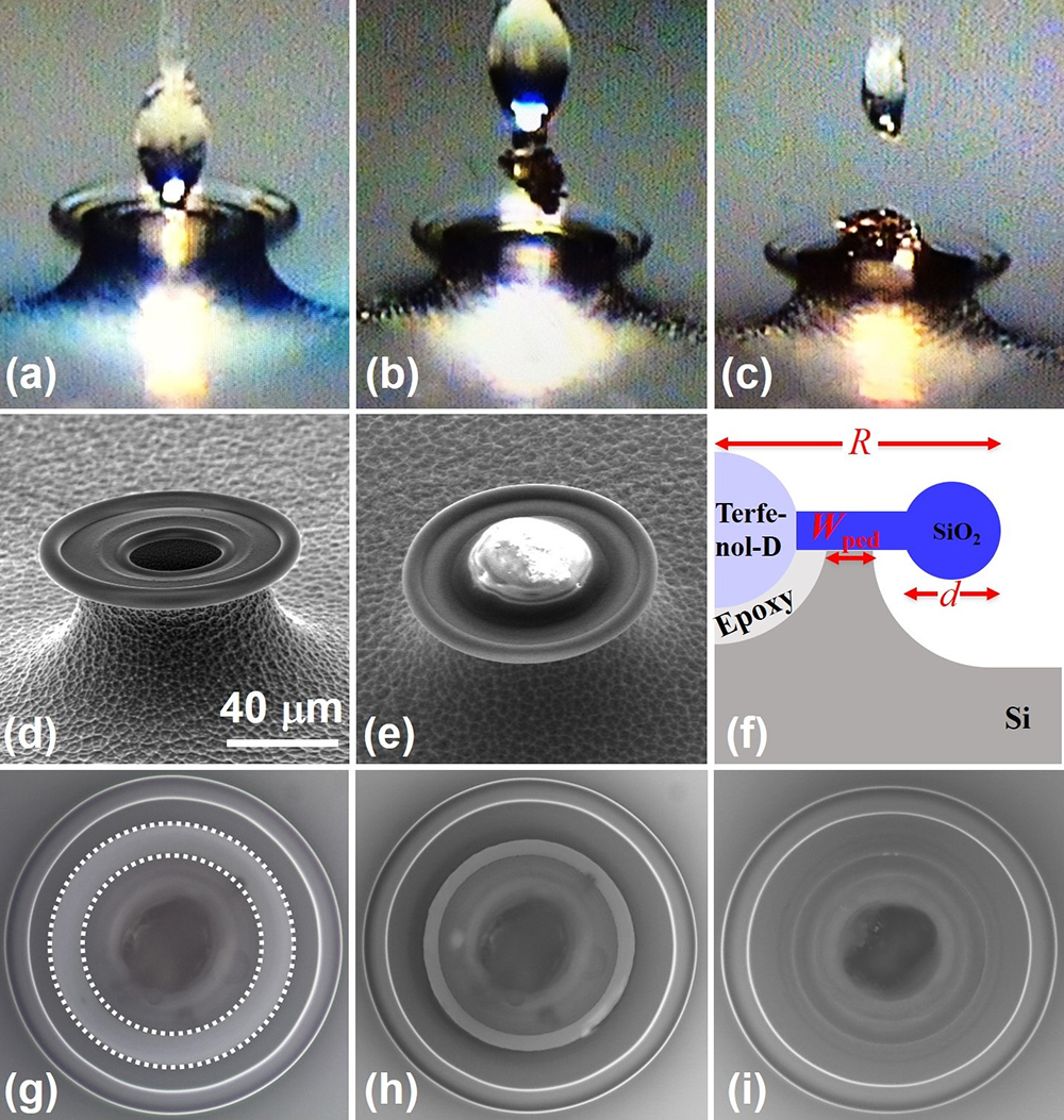
The magnetometers are fabricated by depositing Terfenol-D particles into holes etched into the center of silica microtoroids, following the approach in Ref. [12], as shown in Figs. 1(a)–1(c). The silica microtoroids with central holes are first fabricated through photolithography, hydrofluoric acid etching, xenon difluoride (XeF2) etching, and carbon dioxide (CO2) laser reflow process [28]. We choose the minor diameters in the range of 5–7 μm to maintain high optical quality factors. We then use a fiber tip to deposit a droplet of epoxy into the hole [Fig. 1(a)], and use the same fiber tip to pick up a piece of Terfenol-D and place it into the epoxy inside the hole [Figs. 1(b) and 1(c)]. The epoxy is then cured over a period of 8 h, to provide the bonded magnetometer. Figures 1(d) and 1(e) are scanning electron microscope (SEM) images of one silica microtoroid before and after the Terfenol-D deposition. Figure 1(f) shows a side view schematic of the magnetometer, with a principal radius of R, minor diameter of d, and a pedestal width of Wped.

To measure the magnetic field sensitivity of the fabricated magnetometers, we use a tapered fiber [29] to couple light from a tunable laser in the 1550 nm wavelength band into one of their whispering gallery modes (WGMs). We then use a photoreceiver to detect the light transmitted from the microtoroids back into the tapered optical fiber. After we identify a high-Q WGM, we thermally lock the laser frequency on the blue side of the mode [30]. Mechanical motion due to the applied magnetic field modulates the perimeter of the device and therefore changes the optical resonance. This translates into a periodical modulation in the transmitted light intensity. We use a spectrum analyzer (SA) to measure the noise power spectrum. We then apply a magnetic field to the magnetometer using a coil driven by a network analyzer. This allows the frequency of the magnetic field applied to the magnetometer to be swept and the magnetic response at each frequency to be characterized. With the noise power spectra and system response, we derive the magnetic field sensitivity, following Ref. [11].

In our experiment, to achieve a uniform CO2 laser reflow process, the silicon pedestal is left with a width of ∼5–10μm after the XeF2 etching. Here, in order to improve the mechanical compliance and thus improve the magnetic field sensitivity, we then further etch down the silicon pedestal by performing several runs of XeF2 etching after the Terfenol-D deposition process is complete. The width of the pedestal can be directly measured from an optical microscope image, and is marked in the area between the two white dashed circles in Fig. 1(g). Figures 1(g)–1(i) are optical microscope images of a magnetometer with gradually decreased pedestal width.

We etch down the silicon pedestal by a few microns in each run of XeF2 etching, and measure the sensitivity. In Figs. 2(a) and 2(b), we plot the noise power spectra and sensitivity of a magnetometer with Wped=4.5μm (red curves) and Wped=0.5μm (blue curves), respectively. We find that, as Wped decreases, the mechanical resonances move to lower frequency, due to the increased mechanical compliance and therefore decreased spring constant of the microtoroids. The sensitivity improves across almost the entire active frequency range. In Figs. 2(c) and 2(d), we plot, respectively, the frequency of the peak sensitivity and the peak sensitivity as a function of the pedestal width. The inset of Fig. 2(d) shows optical microscope images of the magnetometers with pedestal widths of 4.5 μm (left) and 0.5 μm (right), respectively. It can be seen that, when the pedestal width is decreased from 4.5 μm to 0.5 μm, the peak sensitivity of the magnetometer is improved from 450pT/Hz at 47.7 MHz to 200pT/Hz at 44.5 MHz. This sensitivity improvement from silicon pedestal etching is consistently observed in most magnetometers. The peak sensitivity could be further improved by increasing the size of the cavity, as discussed in previous work [14].

In Fig. 3, we plot the noise power spectra, system responses, and sensitivity spectra of two magnetometers with pedestal widths less than 5 μm. Characterizing several magnetometers, we observed that they each exhibit one of the two distinct behaviors, as illustrated on the left and right columns of Fig. 3. We define magnetometers that fit into the two classes as Type I and Type II, respectively. For the Type I magnetometer, the magnetic response is relatively smooth as a function of the frequency, with peaks corresponding to the mechanical resonances. Figures 3(a) and 3(b) show the noise power spectrum and the system response of a Type I magnetometer. For Type II magnetometers, in addition to the mechanical resonance peaks, there exists strong modulation of magnetic response as a function of the frequency, as shown in Fig. 3(d). This phenomenon will be further studied in the following section.

The peak sensitivity found for Type I magnetometers is ∼44pT/Hz at about 30 MHz. This frequency corresponds to the radial breathing mode of the magnetometer, with its mode profile shown in the inset of Fig. 3(c), obtained through finite element method simulation using COMSOL Multiphysics. Generally this mode has the largest spatial overlap with the magnetostriction of the Terfenol-D. For the Type II magnetometer, both the magnetic response and sensitivity vary significantly with small changes in the frequency of the magnetic field, as shown in both Figs. 3(e) and 3(f) and in their zoom-ins shown in Figs. 4(a) and 4(b). It can be seen that the magnetic response varies by more than 25 dB within a frequency range of 20 kHz. The peak sensitivity is ∼26pT/Hz, at ∼10.5MHz, and is flat over a 74 kHz frequency band, which is comparable with other high precision magnetometers, such as atomic magnetometers [24,25] and nitrogen vacancy center magnetometers [26,27]. This sensitivity is state of the art in micro-optomechanical systems, and is comparable to the sensitivity of microsized superconducting quantum interference devices (SQUIDs) [21–23]. The sensitivity could be further improved with a thermal-noise-limited sensitivity of around 1pT/Hz, predicted for perfect spatial overlap [11,14]. One approach to improve spatial overlap would be to use the superior structure control available when sputter coating thin films of Terfenol-D as opposed to epoxy bonding [16].

In order to study the two types of magnetic response, we fabricated a total of 26 magnetometers. Of them, we found that 18 exhibited Type I magnetic response, and eight showed Type II magnetic response. In Fig. 5, we plot the peak sensitivities of the 26 magnetometers, with the red squares denoting the Type I magnetometers, and the blue circles the Type II magnetometers. The results in Fig. 3 correspond to device No. 25 (Type I) and No. 9 (Type II), respectively. We note, also, that the Type I magnetometers have a more reliable performance, with five of them having sensitivity better than 100pT/Hz. The average sensitivities of the Type I and Type II magnetometers are 470pT/Hz and 1.1nT/Hz, respectively. One of the contributions to the variance in sensitivity across devices is the anisotropic magnetostriction of Terfenol-D. A possible solution is to apply a DC magnetic field during the fabrication process, which can align the easy magnetic axis of the Terfenol-D particles along the direction of the external magnetic field. This is expected to improve both the reproducibility and the sensitivity of the magnetometers.

All of the measured magnetometers were fabricated using the same method. The fact that magnetic domains in Terfenol-D can have a size similar to size of the grains [31–33] used in our experiment suggests that the two different types of magnetic responses originate from the variations in the number and configurations of the crystal grains. In particular, we postulate that the Terfenol-D particles we used in the Type I and II magnetometers are single crystalline and polycrystalline, respectively. Since the magnetostriction of Terfenol-D is caused by the domain boundary movement in the presence of a DC magnetic field [31], this would mean that the Type II response could be engineered by an external magnetic field. To confirm this, we then take one Type II magnetometer (device No. 26 in Fig. 5) and measure its magnetic response under an external DC magnetic field. In Figs. 6(a) and 6(b), we plot the amplitude and phase of the magnetic response of the magnetometer, measured from the network analyzer, under an external DC magnetic field of ∼93mT. The phase here measures the relative phase between the magnetic response of the magnetometer and the driving field from the network analyzer. Generally, the relative phase changes linearly with frequency. However, there exist multiple abrupt phase changes at the frequencies where the magnetic response exhibits anti-resonance-like dips, with one example shown in the shaded area in Figs. 6(a) and 6(b). As a comparison, for Type I magnetometers abrupt phase changes only occur at the mechanical resonances (not shown here), due to the phase changes of mechanical susceptibilities around the mechanical resonances. In order to study how the amplitude of the DC magnetic field affects the magnetic response of the magnetometer, we gradually decrease the amplitude of the DC magnetic field from 93 mT to 6 mT, with the result shown in Fig. 8(a) in Appendix A. We observe that the magnetic response changes significantly, especially at the frequencies of the dips.

This strong dependence of the magnetic response on the applied DC field observed in Type II magnetometers can be explained by interference between the magnetostrictive waves generated at each crystal grain, with destructive interference responsible for the observed anti-resonance-like dips in the response. To explore this interference effect, we use a simple multiwave interference model to simulate the process. Figures 6(c) and 6(d) show the amplitude and phase of the total response from interference of multiple waves. Multiple dips arise naturally in the response spectrum and abrupt phase changes appear at the dip frequencies, due to the destructive interference of different waves. For more detailed analysis of the Type II magnetic response, see Appendix A and Fig. 8. In order to simulate the effect of changing the amplitude of the applied DC magnetic field, we gradually change the relative amplitude of each wave component (simulating modifications of the magnetostriction coefficient due to an external DC magnetic field), with the result shown in Fig. 8(b) in Appendix A. It can be seen that the depth of the dips in the response spectrum changes significantly, e.g., in the shaded area.

We finally discuss the bandwidths of the magnetometers. Due to the fact that the microtoroids support various mechanical modes in a large frequency range from hundreds of kHz to hundreds of MHz, the magnetometers can detect magnetic fields over a broad bandwidth. As can be seen in Figs. 3(c) and 3(f), the working bandwidths for both Type I (device No. 25 in Fig. 5) and Type II (device No. 9 in Fig. 5) magnetometers exceed 130 MHz, limited by the bandwidth of the photoreceivers we use in the experiment. We define the continuous 3 dB bandwidth to be the frequency range over which the sensitivity is within a factor of 2 of the peak sensitivity. With this definition, we find the continuous 3 dB bandwidth in the range of 10 MHz for Type I magnetometers, considerably larger than that of other types of room-temperature magnetometers, such as atomic magnetometers [24,25] and nitrogen vacancy center magnetometers [26,27], while the continuous bandwidth for Type II magnetometers is typically around 10 kHz, comparable to the full bandwidth of other types of magnetometers [24–27]. In order to quantify the full bandwidth, we use the accumulated bandwidth [15], which quantifies the accumulated frequency range over which the sensitivity is better than a certain threshold value. This is illustrated in the inset of Fig. 7, where the accumulated bandwidth is the total frequency range of the shaded area. In Fig. 7, we plot the accumulated bandwidth for a Type I magnetometer (black curve) and a Type II magnetometer (red curve), as a function of the threshold sensitivity. The 3 dB bandwidth, over which the sensitivity is within a factor of 2 of the peak sensitivity, is obtained to be ∼11.3MHz for the Type I magnetometer, and ∼120kHz for the Type II magnetometer.

In summary, we have achieved an on-chip, room-temperature magnetometer, with a peak sensitivity of 26pT/Hz. This is state of the art for micro-optomechanical magnetometers and is comparable to microscale SQUIDs. We have also found that our magnetometers exhibit two qualitatively different classes of magnetic response. The Type I magnetometers show a relatively smooth magnetic response as a function of the frequency, following the mechanical resonances of the device; while the magnetic response of the Type II magnetometers varies significantly over frequency ranges of 10 kHz, within the envelope of the mechanical resonances. We postulate that magnetometers with single crystalline Terfenol-D particles show a Type I magnetic response, and those with polycrystalline Terfenol-D particles show a Type II magnetic response, and that the dips in the magnetic response spectra of the Type II magnetometers arise due to the destructive interference of the magnetostrictive response from different crystal grains. Finally we show that the optomechanical magnetometers can have an ultrabroad accumulated bandwidth. The working bandwidth exceeds 130 MHz for both the Type I and Type II magnetometers. The 3 dB bandwidth where the sensitivity is within a factor of 2 of the peak sensitivity is found to be ∼11.3MHz for a Type I magnetometer, and ∼120kHz for a Type II magnetometer, respectively, considerably larger than that of other sensitive room-temperature magnetometers. The high sensitivity and broad bandwidth open up new possibilities for applications such as on-chip microfluidic magnetic resonance imaging (MRI).

Acknowledgment. We thank James Bennett, Varun Prakash, Guangheng Wu, and Enke Liu for the very helpful discussions. This work was primarily funded by DARPA QuASAR Program, Australian Research Council, Australian Defence Science and Technology Group, and Commonwealth of Australia as represented by the Defence Science and Technology Group of the Department of Defence. W. P. B. acknowledges an Australian Research Future Fellowship. B. B. L. acknowledges a University of Queensland Postdoctoral Research Fellowship. Device fabrication was performed within the Queensland Node of the Australian Nanofabrication Facility.