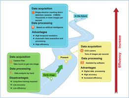
Fig. 1. (Color online) The evolution of TEM data acquisition and processing.

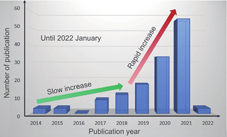
Fig. 2. (Color online) Publications from the Web of Science with the keywords of TEM and machine learning.

Fig. 3. (Color online) Application of artificial intelligence for high-efficient processing of various TEM datasets. FCN, CNN, and UDN are short for fully convolution network, convolutional neural network, and unsupervised deep network, respectively.

Fig. 4. (Color online) The introduction of a neural network in the analysis of atomic defects^[72]. (a) Schematic architecture of a CNN with an encoder-decoder structure. (b) Location of carbon atoms of graphene. (c) The extracted dopant Si atoms and, in this way, the classification between 3-fold and 4-fold Si defects is conducted. (d) The evolution of the same Si dopant on the time scale. (e) Classification of defect types. (f) Extraction of the defect from STEM images.

Fig. 5. (Color online) Introduction of CNN-based algorithm for atomic-scale identification of point and line defects^{[61, 64]}. (a) A CNN as a denoiser process. (b, c) Comparison of the signal-to-noise between the unprocessed and processed images. (d) Defect mapping of STEM image. (e) The statistics of Se vacancies and V dopants change according to the electron beam irradiation time. The scale bar is 5 nm. (f) The architecture of U-Net. (g, h) The border recognition of a nanopore.

Fig. 6. (Color online) Introduction of two machine learning based methods in morphology analysis of gold particles^{[63, 68, 70]}. (a, b) A complete unsupervised clustering algorithm utilized in classification of gold nanorods. (c) A GA containing various image analysis methods as genes to explore the morphological characteristics of NPs. (d) NPs segmented by U-Net with boundaries. (e) The intensity of the four types of NPs and the background in the TEM images explored by U-Net. (f) Boundaries of NPs colored to their local etching rates and the etching time indicate the height. (g) The three etching stages defined by the relationships between the etching rate and curvature.

Fig. 7. (Color online) Application of machine learning based methods in the analysis of atomic column heights. (a) A CNN illustration as an example of the supervised network utilized in the analysis. (b) Comparison between ground truth and prediction after regression and classification on STEM images. (c) Results of the network with various defocus values and electron dose. (d) The sub-unit cell calculated and mapped from a 4D-STEM dataset. (e) Comparison between c-CNN and r-CNN measurement and HAADF estimation.

Fig. 8. (Color online) Application of CNN in structure analysis. (a) The workflow of deploying a neural network model to automatically classify structure. (b–d) Two-dimensional diffraction patterns of different crystal structures are divided into eight classes in SAED. (e) An illustration of a CNN(LeNet-5) with a computer-simulated training dataset. (f) Comparison between manual and automatic classification. (g) Correlation matrix of the results of the two methods.

Fig. 9. (Color online) Introduction of the use of a neural network to explore the correlative laws between local geometries and plasmon responses^[65]. (a) The im2spec network, in which subimages are taken as features and spectra are taken as targets. (b) The spec2im network, which is trained with HAADF spatial descriptors and corresponding spectral descriptors, similar to the im2spec network. However, the spectra are used as features and subimages are used as targets.

Fig. 10. (Color online) The work flow of the 3D construction of STEM energy-dispersive X-ray spectroscopy (STEM-EDX) by deep learning^[67]. (a) Collection of raw EDX experimental maps. (b) A denoising network to improve the noisy EDX maps. (c) Unsupervised deep network to generate high-quality 3D reconstruction.

Table 1. The main parameters of TEM data analysis that is based on machine learning of different types of material properties.