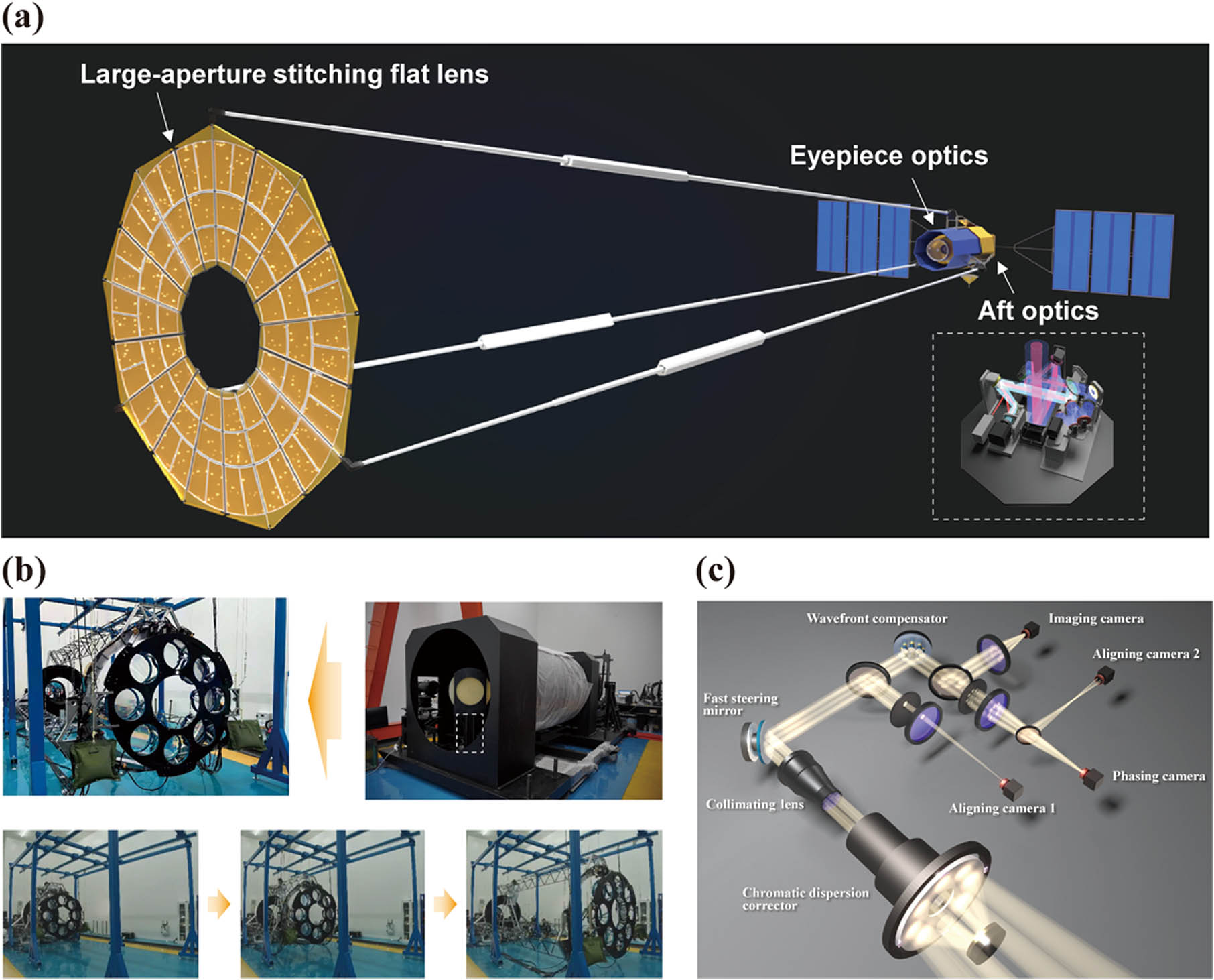
Fig. 1. Ground testbed of the space-based flat imaging system. (a) Schematic of an exemplary space-based giant flat imaging system, including a stitching flat lens with aperture larger than 10 m, eyepiece optics, and aft optics. (b) Ground testbed of a 1.5-m spaceborne stitching flat imaging system. The segmented flat lens is initially folded, then unfurled, and finally stretched. The source is located at the focus of a 1.5-m collimator to simulate objects at infinity. (c) Setup of the aft optics of the 1.5-m flat imaging system. Light cofocused by the seven flat segments is first chromatism-corrected, then collimated, and finally split into the two aligning cameras, the phasing camera, and the imaging camera, respectively.

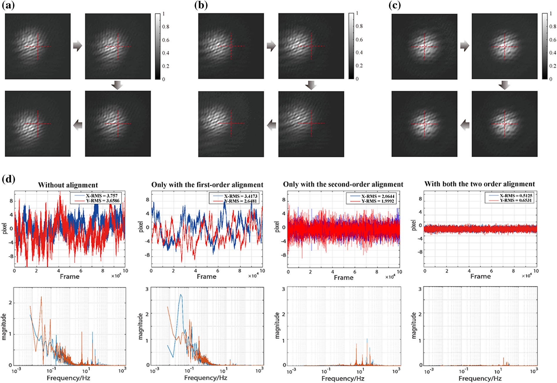
Fig. 2. Results of the two-order tip/tilt alignment. Sequential point spread functions on the phasing camera (a) prior to alignment, (b) with the first-order alignment, and (c) with the two-order alignment. The intensities are normalized with the center of the detector marked by the red cross line. Initially without alignment, the roughly overlapped spots shake randomly. Use of the first-order alignment almost stabilizes the initial mixed spots by rejecting the holistic vibration, but the envelope also slightly varies with the surrounding speckle drifting due to the residual segments’ respective jitters. Joint use of the two-order alignment succeeds in keeping the seven sub-aperture spots stably overlapped and centered on the phasing camera. (d) Disturbance variations of one of the seven defocused spots on the aligning camera 2 in both the time and frequency domains. The magnitude of high-frequency disturbance nearly vanishes only with the first-order alignment and so does that of low-frequency disturbance only with the second-order alignment. The magnitudes of both high- and low-frequency disturbances nearly vanish with the two-order alignment.

Fig. 3. Results of coarse and fine phasing. (a) Sequential point spread functions on the phasing camera during the parallel scanning procedure. Sequential point spread functions on the phasing camera (b) with post coarse phasing and (c) with the loop of fine phasing closed. The spectrum of the white source ranges from 550 to 650 nm. With coarse phasing done, the interference pattern with high-contrast fringes appears but varies with the external disturbance. With fine phasing running, an ideal symmetrical interference pattern owning an obvious peak centered is obtained and maintained against the external disturbance. (d) Wavefront RMS with the closed-loop fine phasing running. The averaged wavefront RMS is 0.053λ (at 600 nm).

Fig. 4. Imaging results of the 1.5-m flat optical system. Direct imagery of a resolution test chart (a) prior to alignment and phasing, (b) post alignment, and (c) with alignment and phasing running. The initial imaging result presents serious ghosting. The imaging clarity is improved with ghosting eliminated by use of alignment. With both the closed-loop alignment and phasing running, the imaging quality is further improved with the resolution bars of each group resolved. (d) Deconvolution image with the contrast and sharpness obviously enhanced.

Fig. 5. Simulation results of phasing a 10 m system. (a) Pupil arrangement of the 10-m stitching flat telescope and (b) nonredundant mask over the 36 pupils designed by an optimization model. (c) Distribution of all the sub-spots on the aligning detector. With the sub-PSFs totally separated on the aligning detector, it is available to sense tip/tilt errors of the 36 segments simultaneously by tracking sub-spot drifts and then realize alignment. (d) PSFs and (e) wavefronts without phasing, with coarse phasing, and with fine phasing, respectively. Coarse phasing yields a PSF with an intensity peak over speckles by correcting the pistons within 20–220 nm. Fine phasing generates an ideal symmetric interference pattern with a dominant peak with the wavefront RMS of 0.0103λ (at 600 nm).

Fig. 6. Cross-section schematic of the piezo mirror mechanism.

Fig. 7. Flowchart of the two-order tip/tilt alignment algorithm.

Fig. 8. Tracking of multiple defocused spots. (a) Direct image on aligning camera 2. (b) Binary image obtained by adaptive image segmentation and image filtering. (c) Multi-spot labeling results. (d) Multi-spot tracking results.

Fig. 9. Disturbance variations of the defocused spots numbered 1–3 on the aligning camera 2 in both the time and frequency domains.

Fig. 10. Disturbance variations of the defocused spots numbered 4–6 on the aligning camera 2 in both the time and frequency domains.

Fig. 11. Summary flowchart of the whole aligning and phasing process.

Fig. 12. Piston variation of each aperture with the closed-loop fine phasing running.