1.5-m flat imaging system aligned and phased in real time

Zongliang Xie; Kaiyuan Yang; Yang Liu; Tianrong Xu; Botao Chen; Xiafei Ma; Yong Ruan; Haotong Ma; Junfeng Du; Jiang Bian; Dun Liu; Lihua Wang; Tao Tang; Jiawei Yuan; Ge Ren; Bo Qi; Hu Yang

doi:10.1364/PRJ.486637

Abstract

Flat optics has been considered promising for constructions of spaceborne imaging systems with apertures in excess of 10 m. Despite recent advances, there are long-existing challenges to perform in-phase stitching of multiple flat optical elements. Phasing the segmented planar instrument has remained at the proof of concept. Here, we achieve autonomous system-level cophasing of a 1.5-m stitching flat device, bridging the gap between the concept and engineering implementation. To do so, we propose a flat element stitching scheme, by manipulating the point spread function, which enables our demonstration of automatically bringing seven flat segments’ tip/tilt and piston errors within the tolerance. With phasing done, the 1.5-m system has become the largest phased planar instrument ever built in the world, to our knowledge. The first demonstration of phasing the large practical flat imaging system marks a significant step towards fielding a 10-m class one in space, also paving the way for ultrathin flat imaging in various remote applications.

1. INTRODUCTION

The growing scientific pursuits, such as the search for birth of stars and signs of life in the universe, require the apertures of optical imaging systems to be large as tens of meters [1]. According to the laws of light reflection and refraction, it is indispensable for lenses and mirrors to be manufactured with curved surfaces to bend light to the focus, resulting in the bottleneck of bulky optical elements [2]. The cost and mass of the curved optics increase approximately by the cube or square of the diameter [3], which brings grand challenges to the construction of giant imaging systems.

Flat optics is being pursued as a promising candidate to reduce the thickness and weight of lenses by arranging micro- or nano-structures on ultrathin substrates to manipulate light waves [4 –12]. In this way, optical components can be recast as ultrathin and lightweight flat devices without loss of imaging quality. The advantages of mass and volume reduction are of keen interest to the next generation space-based giant optical systems, which have the potential to enable mankind to expand and even reform our understanding of the world, by use of the 10 m class apertures. However, it remains challenging to directly fabricate large-scale monolithic flat lenses by typical manufacturing techniques, such as laser direct writing, electron-beam lithography, or focused ion beam [13,14]. To date, the largest metalenses have centimeter-scale apertures [15], while diffractive lenses with diameters on the order of a few decimeters are commonly reported [13]. One approach to overcoming the dilemma is to stitch a number of small planar optical elements fabricated independently to finally form a large collector. For such stitching flat instrument, it is vital to align all the flat segments and control their optical path differences within a fraction of the imaging wavelength, i.e., the process of cophasing. Only in phase can flat segments jointed together realize the high-resolution of the large equivalent aperture.

Up to now, phasing segmented flat imaging systems has remained at the proof-of-concept stage. In the pioneering program named Eyeglass [16], a monolithic 750 mm flat lens is divided into six panels, each thus owning uniform thickness and wedge. The conceptual experiment is performed, where the six segments initially folded up are unfolded and precisely seamed together via positioned fiducials [17]. Then, a 5 m segmented flat prototype is fabricated but is not tested [18], with neither the phasing performance nor the imaging result presented. The following project MOIRE develops a partial flat lens composed of six elements as a 45° wedge of a 5 m version [19 –22]. Being out of phase, the flat imaging brassboard system fails to reach the expected resolution [22]. In Nautilus, a new notional concept of flat detection [23,24], the alignment technology called the Kinematically Engaged Yoke System (KEYS) is proposed and used to manually stitch a conceptual segmented flat lens, made by dividing a monolithic 240 mm one into nine segments [25]. Our group has phased two 352 mm flat lenses manufactured independently, further proving the feasibility of the stitching approach [26]. Recently, the stitching flat metalenses have been demonstrated for constructing large-aperture metasurface-based elements [14,27]. In the simplified demonstrations, the segmented metalens samples are equivalently modeled by masking a large aperture with three small sub-apertures, without any cophasing error considered [14,27].

Sign up for Photonics Research TOC. Get the latest issue of Photonics Research delivered right to you！Sign up now

There are several obstacles to system-level cophasing for the practical giant stitching flat instrument. First, it is inevitable to induce thickness and wedge errors during molding of flat substrates, which are difficult to compensate on the flat plane. Second, stability is critical for the planar segments having long optical paths and suffering from oscillations of the supporting trusses. Last, optical path differences between any two flat sub-apertures also vary with the oscillations. Due to these challenges, although recognized to have the potential to carry out a 10 m class lens, there is not a phased stitching flat imaging system over 1 m, to the best of our knowledge.

To address the above in-phase problems, this paper proposes a point spread function (PSF)-based flat element stitching scheme, bridging the gap between the concept and engineering implementation of the large-aperture segmented flat device. We build a 1.5-m practical flat imaging system comprising seven planar sub-aperture segments. It is the ground version of a space-based flat instrument, of which the planar lens is mainly supported by three suspended deployable trusses. The on-orbit truss deployment is simulated in our laboratory. Then we utilize the PSF-based flat element stitching scheme to phase the 1.5-m engineering planar prototype suffering from serious oscillations. It mainly involves four steps. First, the strategy of compensating manufacture cophasing errors in the backend path is adopted. Second, we develop a two-order pointing correction approach for system stabilization. Third, a parallel scanning technique is proposed to realize fast coarse phasing. Finally, the piston phases within one wavelength are derived from the phase transfer function (PTF) for real-time fine phasing. Correspondingly, the compact and simple aft optics matching the stitching scheme is designed for wavefront sensing and correction, without the use of complex optical elements. We demonstrate system-level autonomous cophasing of the segmented flat imaging system via these efforts. With aligning and phasing done, the 1.5-m device has become the largest phased flat instrument ever built. Also, we note that the proposed PSF-based flat element stitching scheme can be extended to the 10-m version, as verified by simulation. By breaking through the key in-phase problems of giant flat instruments, this work marks a significant step towards launching and fielding a 10-m class one in space, also paving the way for large-aperture ultrathin flat imaging in earth observation and space exploration.

2. SYSTEM OVERVIEW

As illustrated in Fig. 1(a), an exemplary space-based giant flat optical system mainly consists of a stitching flat metasurface [2,15] or diffractive [16] lens with the aperture larger than 10 m, eyepiece vehicle for optics relay, and aft optics for wavefront correction. A 1.5-m flat imaging system following the basic structure has been built in our laboratory, as shown in Fig. 1(b). Eight off-axis flat sub-aperture elements fabricated on the individual planar thin glass substrates are uniformly distributed within the circular ring with the diameter of the outer circle of 1.5 m. They are fabricated by laser direct writing lithography, with four phase steps and 70% efficiency. Each flat segment has an equal diameter of 352 mm, and is equipped with a multi-freedom motion stage for coarse misalignment adjustment. The brace of the secondary mirror of the scene projector (marked by the white box) blocks the beams from entering the bottom sub-aperture so that only seven flat segments are available to test in the ground demonstration.

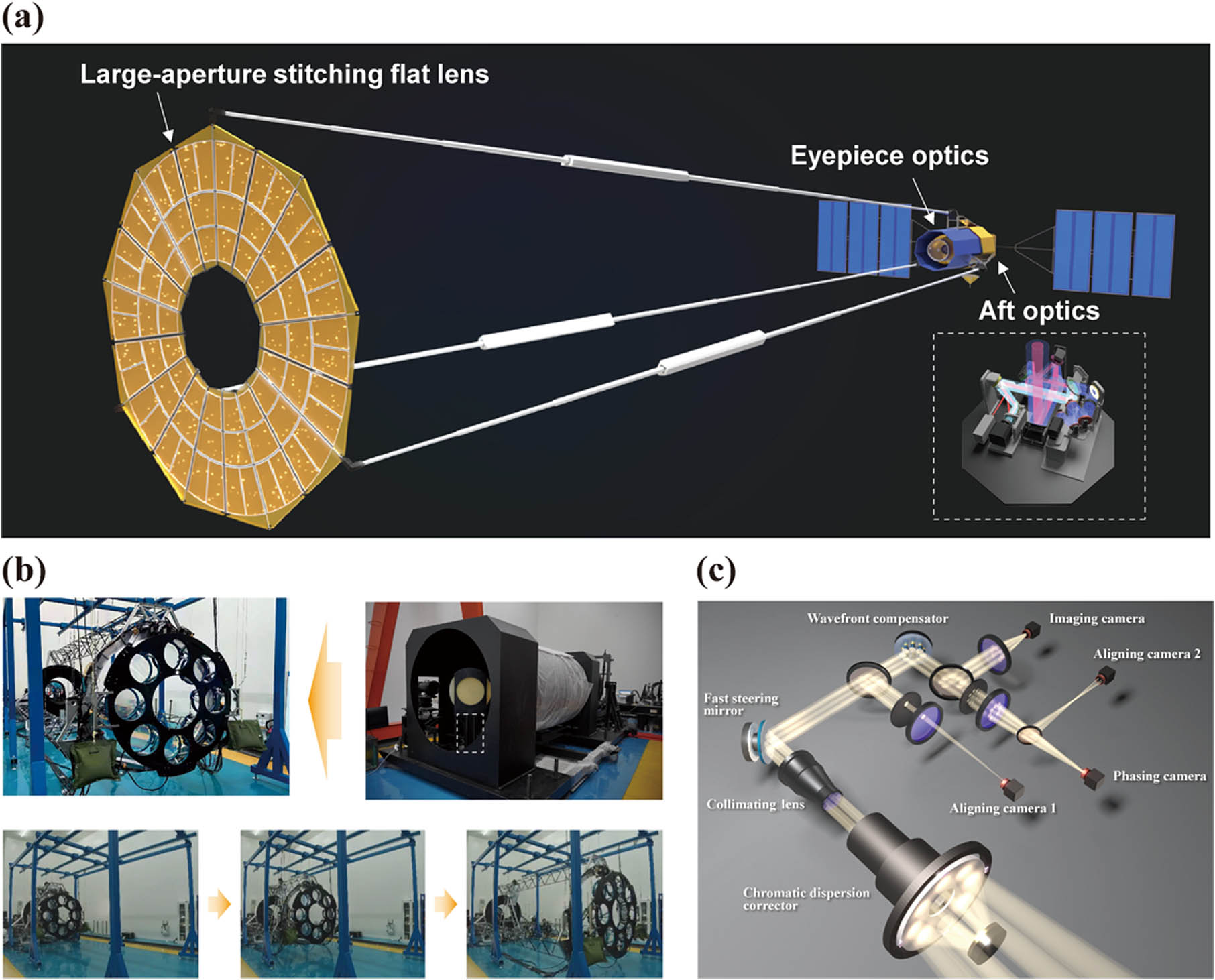
Figure 1.Ground testbed of the space-based flat imaging system. (a) Schematic of an exemplary space-based giant flat imaging system, including a stitching flat lens with aperture larger than 10 m, eyepiece optics, and aft optics. (b) Ground testbed of a 1.5-m spaceborne stitching flat imaging system. The segmented flat lens is initially folded, then unfurled, and finally stretched. The source is located at the focus of a 1.5-m collimator to simulate objects at infinity. (c) Setup of the aft optics of the 1.5-m flat imaging system. Light cofocused by the seven flat segments is first chromatism-corrected, then collimated, and finally split into the two aligning cameras, the phasing camera, and the imaging camera, respectively.

To simulate the commissioning state of the planar observatory spacecraft, we improve the support structure of the flat lens. Unlike the initial version fastened on the bench [26], the updated flat segmented lens is mainly supported by three deployable trusses. To simulate a microgravity condition, the flat lens and trusses are suspended by elastic ropes with sandbags used to balance the weight. In this way, the coaxial locations of the flat lens can be precisely controlled by shrinking and stretching the trusses. The states in which the stitching flat lens is initially folded, then unfurled, and finally stretched are presented in Fig. 1(b). The whole process of pushing out the flat lens, which simulates the operation of the flat observation in space, is exhibited in Visualization 1. During the truss deployment, the elements’ status is monitored by a laser tracking system.

After the flat lens is pushed out to the preassigned position, light coming from the collimator enters. Seven sub-aperture beams are then converged into the eyepiece, which uses a Schupmann achromatic model [28] to overcome the chromatic aberrations in the waveband of 550–650 nm. We have optimized the optics design, generating a corrective field of view of 0.16°. The equivalent focal length of the combination of the flat lens and the eyepiece is 5.4 m. The beams passing through the segmented flat elements and the achromatic module are then collimated into the aft optics exhibited in Fig. 1(c), where wavefront sensing and correction are performed. The details of the aft optics setup can be found in Appendix A.

3. PSF-BASED FLAT ELEMENT STITCHING SCHEME

To realize cophasing of multiple planar sub-apertures, here we propose the PSF-based flat element stitching scheme, which mainly includes four steps.

First, the strategy that cophasing errors are corrected in the backend path is adopted. In conceptual experiments [18,25], the segments are generated from division of one monolithic flat lens, so it is possible to achieve the best optical performance by precisely adjusting the segments’ positions. However, for engineering large-aperture systems, each flat segment needs to be fabricated on an independent substrate. It is inevitable to induce thickness and wedge differences between any two units during the molding of substrates. It is difficult to correct these manufacture errors by adjusting segment positions at the flat plane. Instead, compensating these errors in the aft optics is available. Following the strategy, we develop a wavefront compensator composed of seven piezo mirrors, distributed as the arrangement of flat entrance pupils, as shown in Fig. 1(c). As the core active device, it has triple piezo actuators, allowing for correction of tip/tilt and piston. To compensate for the in-phase errors, the tip/tilt and piston estimates need to be converted to displacements of the three piezo actuators. The conversion principle is described in Appendix B.

Second, we develop a two-order pointing correction approach for stabilization of optical axes. In our ground demonstration, the pointing stability is compromised by the air turbulence, ground vibration, and truss oscillation. During in-orbit operation, the disturbance might come from jitter of the satellite platform, natural vibration of solar arrays, engine running, thermal drift, and so on. We model the disturbance as a combination of high-bandwidth holistic vibration and low-bandwidth segments’ respective drifts. The first-order pointing correction using classical tracking optics aims to restrain the holistic vibration. In the path, a stop is inserted to let only one sub-aperture beam through while blocking the rest. Thus, the global tip/tilt aberrations of the flat segments can be calculated by tracking the shifts of the given PSF on the aligning camera 1 of Fig. 1(c). The second-order pointing correction is employed to overcome the sub-apertures’ respective drifts. In the corresponding path, without the use of Shark–Hartmann sensors [29] or other complex optics [30,31], a CCD detector is simply located at a long defocusing position, where the defocused sub-PSFs are totally separated [32]. The segments’ respective tip/tilt errors can be sensed simultaneously by tracking sub-spot drifts on the aligning camera 2 of Fig. 1(c). The estimates are then fed back to drive the wavefront compensator to correct the tip/tilt aberrations. The details of the two-order tip/tilt alignment algorithms can be seen in Appendix C.

Thirdly, we propose a parallel scanning coarse phasing technique to adjust the initial pistons even larger than the coherence length of the source within one wavelength. The capture range is determined by the actuator’s scanning range. Unlike traditional coarse measurement sensors using complex optics, such as the broadband Hartmann in the Keck telescope [33] and the dispersed Hartmann in JWST [34], the proposed method uses information of the modulation transfer function (MTF), i.e., the amplitude of the PSF’s Fourier transform. Each pair of baselines correspondingly produces a pair of MTF side lobes. Nonredundant pupil distribution can avoid overlap of the MTF side lobes generated by different baselines [35]. In this case, we can command the piston actuators of all the nonreference segments to traverse simultaneously, and at each scanning step calculate the MTF normalized surrounding peak height for each sub-aperture from the PSF captured on the phasing camera of Fig. 1(c). With piston sweep ending, the parallel scanning result can be defined as $M = {[M T F_{n p h - 1}^{T} (x), M T F_{n p h - 2}^{T} (x), \dots, M T F_{n p h - i}^{T} (x)]}^{T}, i = 1, 2, \dots, N,$ (1)where $x$ is the vector of the discrete scanning locations, $M T F_{n p h - i}$ is the vector of the MTF side lobe values corresponding to the $i$ th nonreference sub-aperture, and $N$ is the number of the nonreference sub-apertures. For every baseline, the evolution of the height of the MTF side lobe with respect to pistons can be fitted by the Gaussian function [36,37], so the parallel scanning result can be rewritten as $M \approx {[\exp^{T} (- \frac{{(x - p_{1})}^{2}}{2 σ_{1}^{2}}), \exp^{T} (- \frac{{(x - p_{2})}^{2}}{2 σ_{2}^{2}}), \dots, \exp^{T} (- \frac{{(x - p_{i})}^{2}}{2 σ_{i}^{2}})]}^{T}, i = 1, 2, \dots, N,$ (2)where $p_{i}$ is the initial piston between the $i$ th nonreference sub-aperture and the reference, and $σ_{i}$ is the fitting parameter for the $i$ th nonreference sub-aperture. All the initial pistons of the nonreference sub-apertures can be estimated simultaneously from $p_{coarse} \approx [\max (m^{1}), \max (m^{2}), \dots, \max (m^{i})], i = 1, 2, \dots, N,$ (3)with $m^{i}$ the $i$ th row of $M$ . The fitting deviation might cause whole-wave errors. Repeated running could reduce the probability [37]. Also, the wide working spectrum corresponding to the narrow Gaussian distribution would improve the fitting accuracy and antinoise capability.

Finally, the analytical piston sensing method is adopted for fine phasing and works in a closed-loop manner to maintain the in-phase state during disturbance. The piston error within $\pm 1 / 2$ wave can be extracted from the PTF, i.e., the phase of the PSF’s Fourier transform. Specifically, for every baseline, the PTF value at the positions of the MTF side lobe is exactly the piston between the corresponding pair of sub-pupils [38]. Thus, with nonredundant pupil fragmenting, all the fine pistons of the nonreference sub-apertures can be obtained as $p_{fine} = [{PTF}_{ph - 1}, {PTF}_{ph - 2}, \dots, {PTF}_{ph - i}], i = 1, 2, \dots, N .$ (4)

The aft optics matching the proposed PSF-based flat element stitching scheme is designed, as illustrated in Fig. 1(c). It can be seen that only three common imaging paths, each simply consisting of a mask, lens, and camera, are enough to detect the aberrations. Without use of complex elements such as the prism array [33] and multiple grisms [34], we realize as simple a design as possible. This concision can contribute to stable in-orbit operations of the space observatory.

4. RESULTS AND DISCUSSION

A. In-Phase Stitching of the 1.5-m Flat Imaging System

The PSF-based flat element stitching scheme is utilized to automatically align and phase the flat imaging system. The NKT supercontinuum laser located at the focal plane of the 1.5-m collimator serves as the white light source, simulating a bright star at infinity. The central wavelength is selected as 600 nm with the bandwidth set to be 100 nm.

To start with, the flat lens is pushed out to match the focal length by stretching the trusses. With the flat segments arriving at the preassigned positions, coarse adjustment is conducted to roughly converge the seven sub-aperture spots. As noted, in our ground demonstration, the system suffers from air turbulence, ground vibration, and truss oscillation. Thus, the roughly overlapped spots on the phasing camera shake randomly, as shown in Fig. 2(a), where the intensities are normalized with the center of the detector marked by the red cross line to clearly exhibit the variation of spot positions. Then we perform the first-order alignment, almost stabilizing the initial mixed spots with the holistic vibration rejected, as shown in Fig. 2(b). However, due to the residual segments’ respective drifts, the envelope of the mixed spots slightly varies with the surrounding speckle drifting, which calls for an additional alignment. Before performing the second-order alignment, we calibrate the reference positions for defocused sub-aperture PSFs, as described in Appendix D. Then the wavefront compensator is commanded in the closed-loop manner to fix the seven defocused spots to their respective calibrated positions on the aligning camera 2, thus keeping the seven focused spots being stably overlapped and centered on the phasing camera, as presented in Fig. 2(c). The whole procedure of the two-order pointing correction is displayed in Visualization 2.

Figure 2.Results of the two-order tip/tilt alignment. Sequential point spread functions on the phasing camera (a) prior to alignment, (b) with the first-order alignment, and (c) with the two-order alignment. The intensities are normalized with the center of the detector marked by the red cross line. Initially without alignment, the roughly overlapped spots shake randomly. Use of the first-order alignment almost stabilizes the initial mixed spots by rejecting the holistic vibration, but the envelope also slightly varies with the surrounding speckle drifting due to the residual segments’ respective jitters. Joint use of the two-order alignment succeeds in keeping the seven sub-aperture spots stably overlapped and centered on the phasing camera. (d) Disturbance variations of one of the seven defocused spots on the aligning camera 2 in both the time and frequency domains. The magnitude of high-frequency disturbance nearly vanishes only with the first-order alignment and so does that of low-frequency disturbance only with the second-order alignment. The magnitudes of both high- and low-frequency disturbances nearly vanish with the two-order alignment.

We then quantitatively evaluate the performance of the two-order alignment scheme. The disturbance variations of one of the seven defocused spots on the aligning camera 2 are plotted in Fig. 2(d). As can be seen, before alignment the vibration causes the chosen spot to shake randomly, with RMS values of the centroid shifts of 3.757 and 3.659 pixels along the $X$ and $Y$ axes, respectively. The first-order alignment restrains the holistic vibration, which mainly causes high-frequency disturbance. It can be seen that with the holistic vibration rejected by the first-order alignment, the high-frequency burr of the curve of centroid shifts is removed. The RMS values are reduced to 3.4173 and 2.6481 pixels. We note that after the first-order alignment the RMS values might also be increased with segments’ respective drifts intensified. The corresponding results are presented in Appendix E. When only the second-order alignment operates, the disturbance can be mitigated better, yet with residual centroid shifts left, of which the RMS values are 2.064 and 1.999 pixels in the $X$ and $Y$ axes, respectively. The reason is that the correction bandwidth is limited. Only by performing both the two-order alignment can the disturbance be completely suppressed with stabilization accuracy of 0.513 and 0.653 pixels for the $X$ and $Y$ directions, respectively. From the analysis in the frequency domain, it can be intuitively recognized that the first-order alignment corrects for high-frequency disturbance over about 4 Hz caused by the holistic vibration that all the seven sub-apertures suffer from, while the second one corrects for low-frequency disturbance induced by the sub-apertures’ respective drifts. The disturbance at both high and low frequencies can be rejected by joint use of the two-order alignment. The disturbance variations of the other six defocused spots on the aligning camera 2 present the similar results, which are also illustrated in Appendix E.

It is ready to start the phasing process during the implementation of the two-order alignment. The parallel scanning coarse phasing technique is first performed. The piston actuators of all the six nonreference segments are commanded to traverse parallelly, and sequential PSFs are captured. The scanning range is $\pm 6 μm$ with a step of 30 nm. The parallel scanning procedure is briefly shown in Fig. 3(a). A wide range of pistons are estimated from the parallel scanning results and drive the wavefront compensator to perform corresponding correction. With coarse phasing done, the seven sub-aperture beams interfere with each other obviously, generating high-contrast fringes shown in Fig. 3(b). Specifically, right after coarse phasing ends, an approximately symmetric interference pattern with a peak appears. However, as the external disturbance induces variations of the optical path lengths, the indistinct interference peak disappears and the speckle-like patterns vary randomly. Fine phasing in a closed-loop manner is capable of compensating the transient optical path length differences. Before operation of fine phasing, coarse phasing is needed again to reduce the probability of whole-wave errors. Since the first coarse phasing has shortened the pistons, the second scanning range is reduced to $\pm 2 μm$ . Once the second coarse phasing is done, the loop of fine phasing is closed. As shown in Fig. 3(c), the transient interference pattern generated by fine phasing is distributed symmetrically with an obvious peak centered. This ideal interference state is maintained during the external disturbance. The whole procedure of both coarse and fine phasing is exhibited in Visualization 2. The summary flowchart of the whole aligning and phasing process is shown in Appendix F. Because there is no truth sensor, we approximately calculate RMS values of wavefront from PTF estimates of 1000 frames of PSFs with closed-loop fine phasing, which are presented in Fig. 3(d). The piston variation of each aperture with fine phasing can be seen in Appendix G. With the closed-loop fine phasing running, the averaged RMS is $0.053 λ$ wave at 600 nm central wavelength.

Figure 3.Results of coarse and fine phasing. (a) Sequential point spread functions on the phasing camera during the parallel scanning procedure. Sequential point spread functions on the phasing camera (b) with post coarse phasing and (c) with the loop of fine phasing closed. The spectrum of the white source ranges from 550 to 650 nm. With coarse phasing done, the interference pattern with high-contrast fringes appears but varies with the external disturbance. With fine phasing running, an ideal symmetrical interference pattern owning an obvious peak centered is obtained and maintained against the external disturbance. (d) Wavefront RMS with the closed-loop fine phasing running. The averaged wavefront RMS is $0.053 λ$ (at 600 nm).

During the closed-loop alignment and phasing using the point source, a conjugated resolution test chart illuminated by a halogen bulb is projected onto the imaging camera. Figure 4(a) is the imaging result prior to alignment and phasing, presenting serious ghosting. Use of alignment improves the clarity of the image by eliminating ghosting but fails to resolve the resolution texture, as shown in Fig. 4(b). With both the closed-loop alignment and phasing running, a synthetic image presented in Fig. 4(c) is obtained, where the resolution bars of each group can be almost resolved, though suffering from air turbulence. We then perform a deconvolution on the result, obtaining a high-resolution processed image with the contrast and sharpness obviously enhanced, as shown in Fig. 4(d). The minimum line width (group 36) of the resolution test chart used here is 7.07 μm, corresponding to the angle resolution of 0.94 μrad. Here we use optical-path-splitting sensing for simultaneous imaging of the point source and test chart. The deviation between the reflected and transmitted wavefronts of the beamsplitter used to divide the phasing and imaging paths might decrease the imaging quality. Designing and fabricating a beamsplitter with high optics quality could further improve the direct imagery.

Figure 4.Imaging results of the 1.5-m flat optical system. Direct imagery of a resolution test chart (a) prior to alignment and phasing, (b) post alignment, and (c) with alignment and phasing running. The initial imaging result presents serious ghosting. The imaging clarity is improved with ghosting eliminated by use of alignment. With both the closed-loop alignment and phasing running, the imaging quality is further improved with the resolution bars of each group resolved. (d) Deconvolution image with the contrast and sharpness obviously enhanced.

B. Simulation of Phasing a 10-m Flat Imaging System

When the flat stitching lens scales to a 10 m class one, tens of planar sub-aperture segments are needed. We note that regardless of the sub-aperture numbers and configurations, the proposed PSF-based flat element stitching scheme is also applicable to the 10 m class version, if a proper nonredundant mask over dozens of pupils is designed.

Here we perform a simulation demonstration. A simulated stitching flat telescope composed of 36 segments is built with the aperture of 10 m, as shown in Fig. 5(a). The imaging wavelength ranges from 550 to 650 nm. The diameter of each unit is 1.35 m. The F-number is 21.3, the same as that of the 1.5 m prototype. The key to using the PSF-based flat element stitching scheme to phase the dozens of pupils is the design of a nonredundant mask. The increase of the segment numbers results in the increase of the design difficulty of nonredundant distribution. To address this problem, we propose an optimization model as follows: $\underset{P, Q}{\arg \max} \sum_{i = 1}^{N} (ε (\min ({‖ P_{i} Q_{j, k} ‖}_{2}) - \frac{D}{2 λ f})), j = 1, 2, \dots, N - 1, k = j + 1, j + 2, \dots, N,$ (5)where $P_{i}$ represents the coordinates of the MTF side lobe formed by the $i$ th nonreference pupil and the reference one, $Q_{j, k}$ represents the coordinates of the MTF side lobe formed by the $j$ th and $k$ th nonreference pupils, $λ$ is the wavelength, $D$ is the sub-pupil diameter, $f$ is the focal length, and $ε (\cdot)$ is the step function. With the distance between $P_{i}$ and $Q_{j, k}$ larger than $D / 2 λ f$ , the overlap of the $P_{i}$ MTF side lobe can be avoided. Then we perform the genetic algorithm to maximize the metric function, automatically generating a nonredundant mask shown as Fig. 5(b).

Figure 5.Simulation results of phasing a 10 m system. (a) Pupil arrangement of the 10-m stitching flat telescope and (b) nonredundant mask over the 36 pupils designed by an optimization model. (c) Distribution of all the sub-spots on the aligning detector. With the sub-PSFs totally separated on the aligning detector, it is available to sense tip/tilt errors of the 36 segments simultaneously by tracking sub-spot drifts and then realize alignment. (d) PSFs and (e) wavefronts without phasing, with coarse phasing, and with fine phasing, respectively. Coarse phasing yields a PSF with an intensity peak over speckles by correcting the pistons within 20–220 nm. Fine phasing generates an ideal symmetric interference pattern with a dominant peak with the wavefront RMS of $0.0103 λ$ (at 600 nm).

With the segments masked nonredundantly, the PSF-based flat element stitching scheme is used to phase the 36 units. From Fig. 5(c), it can be seen that the sub-PSFs are totally separated on the aligning detector, which is simply located at the defocusing position of 3 cm. Thus, it is available to sense tip/tilt errors of the 36 segments simultaneously by tracking sub-spot drifts and then realize alignment. Then, the pistons ranging from 680 to 8700 nm are loaded on the system. The PSFs during piston correction, specifically without phasing, post coarse phasing, and with fine phasing, are presented in Fig. 6(d), respectively. The corresponding wavefronts are shown in Fig. 6(e). Due to the large pistons, there are random speckles in the initial PSF. With coarse phasing done, the pistons are corrected within 20–220 nm, yielding an intensity peak over speckles. With fine phasing, the wavefront RMS becomes $0.0103 λ$ (at 600 nm). The ideal symmetric interference pattern with a dominant peak is then obtained. From this simulation, it is demonstrated that the proposed PSF-based flat element stitching scheme is effective in phasing the 10-m class flat imaging system.

Figure 6.Cross-section schematic of the piezo mirror mechanism.

5. CONCLUSION

In this paper, we try to promote the concept of the large-aperture flat optics towards engineering implementation. We have built a 1.5-m planar optical system consisting of seven flat elements with its mount connected to three deployable trusses. The procedure of stretching the flat lens of the observation in space is simulated in our laboratory. After that, the seven flat sub-apertures suffer from serious external disturbance. The PSF-based flat element stitching scheme involving solutions in both hardware and software is proposed and succeeds in automatically aligning and phasing the flat system. With aligning and phasing done, the 1.5-m planar system has become the largest phased flat instrument ever built in the world, to the best of our knowledge.

Regardless of the sub-aperture numbers and configurations, the PSF-based flat element stitching scheme is also applicable to the 10-m class planar instrument, as verified by simulation. As for engineering implementation of phasing a 10-m class flat device, for the aft optics, the wavefront compensator needs to be updated to enable adjustment of tip/tilt and piston for tens of flat sub-apertures. For alignment, what mainly needs to be done is just to enlarge the window of the detector for the second-order alignment to contain all the defocused spots. For both coarse and fine phasing, in theory, the key problem is to design a nonredundant mask over dozens of pupils, which has been solved here by proposing an optimization framework capable of automatically generating a nonredundant distribution. From both simulation demonstration and feasibility analysis, it is believable that the proposed PSF-based flat element stitching scheme would be effective for phasing the 10-m class planar instrument. With the in-phase challenges of the large-aperture flat optics addressed in this paper, our group plans to build a practical 10-m scale planar optical instrument, and aims at launching and fielding it in space in the future.

APPENDIX A: DETAILS OF THE AFT OPTICS SETUP

The wavefront compensator is composed of seven active mirrors, distributed as the arrangement of the flat sub-aperture segments. Each mirror has triple piezo actuators, allowing for control of the tip/tilt and piston. The resolution and range for piston adjustment are 2 nm and 50 μm, respectively, while for tip/tilt being 0.1 μrad and 10 mrad, respectively. The resonant frequency is more than 1000 Hz.

128 \times 128 pixels

512 \times 512 pixels

128 \times 128 pixels

APPENDIX B: CONVERSION BETWEEN TIP/TILT/PISTON AND PIEZO DISPLACEMENTS

A

{(\begin{matrix} α \\ β \\ Z \end{matrix})}_{beam} = Q \cdot {(\begin{matrix} A \\ B \\ C \end{matrix})}_{m irror} = (\begin{matrix} \frac{2}{\sqrt{3} b} & - \frac{1}{\sqrt{3} b} & - \frac{1}{\sqrt{3} b} \\ 0 & \frac{1}{b} & - \frac{1}{b} \\ \frac{1}{3} & \frac{1}{3} & \frac{1}{3} \end{matrix}) {(\begin{matrix} A \\ B \\ C \end{matrix})}_{m irror},

APPENDIX C: TWO-ORDER TIP/TILT ALIGNMENT ALGORITHMS

Tip/tilt errors manifest themselves as spot shifts on the two aligning cameras. Here the centroid extraction algorithms combined with the servo-control framework are used to measure and eliminate these shifts.

In the first-order pointing correction, one of the seven beams is selected, of which the shifts characterize the holistic vibration. It is actually a classical fine tracking scheme. The flowchart of the first-order alignment algorithm is presented in the left of Fig. 7 . By extracting the positions of the single spot from the binary image yielded by image segmentation, the global tip/tilt can be easily obtained. The error signal is sent to a PID control loop to drive FSM to stabilize the spot at the center of the aligning camera 1. A more complex controller using error-based observation has been developed in case the disturbance magnitude outruns the capacity of the PID controller [39].

Figure 7.Flowchart of the two-order tip/tilt alignment algorithm.

Figure 8.Tracking of multiple defocused spots. (a) Direct image on aligning camera 2. (b) Binary image obtained by adaptive image segmentation and image filtering. (c) Multi-spot labeling results. (d) Multi-spot tracking results.

An image can be the 4-connected neighborhood or 8-connected neighborhood. In this module, considering computational space and efficiency, we utilize the line-labeling method (LLM) based on 8-connectivity.

c_{x} = \frac{\sum_{x} \sum_{y} x f (x, y)}{\sum_{x} \sum_{y} f (x, y)}, c_{y} = \frac{\sum_{x} \sum_{y} y f (x, y)}{\sum_{x} \sum_{y} f (x, y)},

According to the positions and pupil distribution, the mapping table matching the spots and their corresponding sub-apertures is established, labeling the spot positions with the segment numbers, as shown in Fig. 8 (c). Then stable multi-spot tracking can be realized by repeating the operation on each frame of image, as shown in Fig. 8 (d).

The spot shifts of the seven sub-apertures representing their tip/tilt errors are sent to seven PID control loops, actuating the seven piezo mirrors to stabilize the corresponding spots at their calibrated positions on the aligning camera 2.

APPENDIX D: CALIBRATION OF THE SECOND-ORDER ALIGNMENT

A process of calibration needs to be run before the implementation of the second-order alignment. This is done by actuating the electronic shutters, which are attached to the mask. One of the segments is opened with the others closed off. The second-order closed-loop control only for the open sub-aperture operates, stabilizing both the corresponding defocused spot on the aligning camera 2 and the focused one on the phasing camera. The stabilized position of the former is adjusted until the latter is located at the phasing detector center. Once done, the coordinates of the defocused spot centroid on the aligning detector are recorded as the calibrated position for the open segment. The calibration proceeds until all the seven aligned positions are obtained.

APPENDIX E: ADDITIONAL RESULTS OF THE TWO-ORDER TIP/TILT ALIGNMENT

X

Figure 9.Disturbance variations of the defocused spots numbered 1–3 on the aligning camera 2 in both the time and frequency domains.

Figure 10.Disturbance variations of the defocused spots numbered 4–6 on the aligning camera 2 in both the time and frequency domains.

X

X

X

X

APPENDIX F: SUMMARY FLOWCHART OF THE WHOLE ALIGNING AND PHASING PROCESS

Figure 11 describes the whole aligning and phasing process. First, the first-order alignment corrects the global tip/tilt of the flat segments in a closed control loop. Second, the second-order alignment runs to correct the segments’ respective tip/tilt errors in another closed control loop. During the implementation of the two-order alignment, the coarse phasing scanning is performed twice. Finally, the closed-loop fine phasing runs.

Figure 11.Summary flowchart of the whole aligning and phasing process.

Figure 12.Piston variation of each aperture with the closed-loop fine phasing running.

APPENDIX G: PISTON VARIATION OF EACH APERTURE WITH FINE PHASING

0.052 λ

References

[1] R. Gilmozzi. Giant telescopes of the future. Sci. Am., 294, 64-71(2006).

[2] X. Luo. Subwavelength artificial structures: opening a new era for engineering optics. Adv. Mater., 31, 1804680(2018).

[3] H. P. Stahl. Survey of cost models for space telescopes. Opt. Eng., 49, 053005(2010).

[4] S. Banerji, M. Meem, A. Majumder, F. G. Vasquez, B. Sensale-Rodriguez, R. Menon. Imaging with flat optics: metalenses or diffractive lenses. Optica, 6, 805-810(2019).

[5] J. E. M. Whitehead, A. Zhan, S. Colburn, L. Huang, A. Majumdar. Fast extended depth of focus meta-optics for varifocal functionality. Photon. Res., 10, 828-833(2022).

[6] H. Gao, Y. Wang, X. Fan, B. Jiao, T. Li, C. Shang, C. Zeng, L. Deng, W. Xiong, J. Xia, M. Hong. Dynamic 3D meta-holography in visible range with large frame number and high frame rate. Sci. Adv., 6, eaba8595(2020).

[7] T. D. Milster, Y. S. Kim, Z. Wang, K. Purvin. Multiple-order diffractive engineered surface lenses. Appl. Opt., 59, 7900-7906(2020).

[8] N. Yu, P. Genevet, M. A. Kats, F. Aieta, J. P. Tetienne, F. Capasso, Z. Gaburro. Light propagation with phase discontinuities: generalized laws of reflection and refraction. Science, 334, 333-337(2011).

[9] A. U. R. Khalid, F. Feng, N. Ullah, X. Yuan, M. G. Somekh. Exploitation of geometric and propagation phases for spin-dependent rational-multiple complete phase modulation using dielectric metasurfaces. Photon. Res., 10, 877-885(2022).

[10] L. Kang, H. Bao, D. H. Werner. Interference-enhanced optical magnetism in surface high-index resonators: a pathway toward high-performance ultracompact linear and nonlinear meta-optics. Photon. Res., 7, 1296-1305(2019).

[11] D. Neshev, I. Aharonovich. Optical metasurfaces: new generation building blocks for multi-functional optics. Light Sci. Appl., 7, 58(2018).

[12] H. Gao, X. Fan, W. Xiong, M. Hong. Recent advances in optical dynamic meta-holography. Opto-Electron. Adv., 4, 210030(2021).

[13] H. Zhang, H. Liu, W. Xu, Z. Lu. Large aperture diffractive optical telescope: A review. Opt. Laser Technol., 130, 106356(2020).

[14] F. Zhao, Z. Shen, D. Wang, B. Xu, X. Chen, Y. Yang. Synthetic aperture metalens. Photon. Res., 9, 2388-2397(2021).

[15] L. Zhang, S. Chang, X. Chen, Y. Ding, M. T. Rahman, Y. Duan, M. Stephen, X. Ni. High-efficiency, 80-mm aperture metalens telescope. Nano Lett., 23, 51-57(2023).

[16] R. Hyde. Eyeglass. 1.Very large aperture diffractive telescopes. Appl. Opt., 38, 4198-4212(1999).

[17] R. Hyde, S. Dixit, A. Weisberg, M. Rushford. Eyeglass: a very large aperture diffractive space telescope. Proc. SPIE, 4849, 28-39(2002).

[18] J. Early, R. Hyde, R. Baron. Twenty meter space telescope based on diffractive Fresnel lens. Proc. SPIE, 5166, 148-156(2004).

[19] P. Atcheson, C. Stewart, J. Domber, K. Whiteaker, J. Cole, P. Spuhler, A. Seltzer, J. A. Britten, S. N. Dixit, B. Farmer, L. Smith. MOIRE-initial demonstration of a transmissive diffractive membrane optic for large lightweight optical telescopes. Proc. SPIE, 8442, 844221(2012).

[20] J. A. Britten, S. N. Dixit, M. DeBruyckere, D. Steadfast, J. Hackett, B. Farmer, G. Poe, B. Patrick, P. D. Atcheson, J. L. Domber, A. Seltzer. Large-aperture fast multilevel Fresnel zone lenses in glass and ultrathin polymer films for visible and near-infrared imaging applications. Appl. Opt., 53, 2312-2316(2014).

[21] P. Atcheson, J. Domber, K. Whiteaker, J. A. Britten, S. N. Dixit, B. Farmer. MOIRE: ground demonstration of a large aperture diffractive transmissive telescope. Proc. SPIE, 9143, 91431W(2014).

[22] J. L. Domber, P. Atcheson, J. Kommers. MOIRE: ground test bed results for a large membrane telescope. Spacecraft Structures Conference, 1510(2014).

[23] D. Apai, T. D. Milster, D. W. Kim, A. Bixel, G. Schneider, R. Liang, J. Arenberg. A thousand earths: a very large aperture, ultralight space telescope array for atmospheric biosignature surveys. Astron. J., 158, 83(2019).

[24] D. W. Kim, H. Choi, T. Brendel, H. Quach, M. Esparza, H. Kang, Y. Feng, J. N. Ashcraft, X. Ke, T. Wang, E. S. Douglas. Advances in optical engineering for future telescopes. Opto-Electron. Adv., 4, 210040(2021).

[25] M. A. Esparzaa, H. Choia, D. W. Kim. Alignment of multi-order diffractiv engineered (mode) lens segments using the kinematically-engaged yoke system. Proc. SPIE, 11487, 114870V(2020).

[26] Y. Liu, Z. Xie, H. Ma, J. Chu, X. Ma, Y. Tan, D. Liu, J. Bian, H. Hu, B. Fan, B. Qi. Wide-band high-resolution synthetic imaging of a segmented large-scaled lightweight diffractive telescope. Opt. Lett., 45, 1790-1793(2020).

[27] Y. Lin, Y. Dong, T. Sun, Y. Zhao, M. Wang, J. Hu, C. Wang, Z. Zeng, C. Jiang. High-efficiency optical sparse aperture metalens based on GaN nanobrick array. Adv. Opt. Mater., 10, 2102756(2022).

[28] L. Schupmann. Die medial-fernrohre: eine neue konstruktion für grosse astronomische instrumente(1899).

[29] B. Li, W. Yu, M. Chen, J. Tang, H. Xian. Co-focus experiment of segmented mirror. Chin. Phys. B, 26, 060706(2017).

[30] S. Robbe, B. Sorrente, F. Cassaing, Y. Rabbia, G. Rousset, L. Dame, P. Cruzalebes, G. Schumacher. Active phase stabilization at the I2T: implementation of the ASSI table. Proc. SPIE, 2200, 222-230(1994).

[31] J. Xue, A. Jiang, S. Wang, J. Wang. Design and experimental demonstration of pointing correction module for a Fizeau imaging interferometer. Appl. Opt., 57, 9936-9943(2018).

[32] W. Lv, Z. Xie, Q. Wang, H. Ma, J. Shi, Y. Liu, K. Yang, B. Chen, Y. Huang. Tip/tilt alignment for a Fizeau interferometer via defocus-based sub-spot separation. IEEE Photon. J., 12, 3901113(2020).

[33] G. Chanan, M. Troy, F. Dekens, S. Michaels, J. Nelson, T. Mast, D. Kirkman. Phasing the mirror segments of the Keck telescopes: the broadband phasing algorithm. Appl. Opt., 37, 140-155(1998).

[34] F. Shi, B. M. King, N. Sigrist, S. A. Basinger. NIRCam long wavelength channel grisms as the dispersed fringe sensor for JWST segment mirror coarse phasing. Proc. SPIE, 7010, 70102E(2008).

[35] W. Zhao, Q. Zeng. Simultaneous multi-piston measurement method in segmented telescopes. Opt. Express, 25, 24540-24552(2017).

[36] J. F. Simar, Y. Stockman, J. Surdej. Single-wavelength coarse phasing in segmented telescopes. Appl. Opt., 54, 1118-1123(2015).

[37] M. Ni, L. Benson, J. Camp, B. Herman. Autonomous tip/tilt alignment and phasing of a distributed aperture imaging testbed. Opt. Express, 18, 13051-13056(2010).

[38] D. Mourard, W. Dali Ali, A. Meilland, N. Tarmoul, F. Patru, J. M. Clausse, P. Girard, F. Hénault, A. Marcotto, N. Mauclert. Group and phase delay sensing for cophasing large optical arrays. Mon. Not. R. Astron. Soc., 445, 2082-2092(2014).

[39] Y. Ruan, T. Xu, Y. Liu, Z. Xie, H. Ma, J. Du, T. Yang, T. Tang, H. Yang, Z. Peng. Error-based observation control of an image-based control loop for disturbance suppression in segmented lightweight large-scaled diffractive telescope (SLLDT). Opt. Laser Eng., 156, 107105(2022).