Modeling of three-dimensional exciplex pumped fluid Cs vapor laser with transverse and longitudinal gas flow

Chenyi Su; Xingqi Xu; Jinghua Huang; Bailiang Pan

doi:10.1017/hpl.2021.8

Journals >High Power Laser Science and Engineering >Volume 9 >Issue 2 >Page 02000e26 > Article

High Power Laser Science and Engineering
Vol. 9, Issue 2, 02000e26 (2021)

Modeling of three-dimensional exciplex pumped fluid Cs vapor laser with transverse and longitudinal gas flow

Chenyi Su¹, Xingqi Xu^1,2, Jinghua Huang¹, and Bailiang Pan^1,*

Author Affiliations

¹Department of Physics, Zhejiang University, Hangzhou310027, China

²Interdisciplinary Center for Quantum Information, State Key Laboratory of Modern Optical Instrumentation, and Zhejiang Province Key Laboratory of Quantum Technology and Device, Department of Physics, Zhejiang University, Hangzhou310027, China

show less

DOI: 10.1017/hpl.2021.8 Cite this Article Set citation alerts

Chenyi Su, Xingqi Xu, Jinghua Huang, Bailiang Pan, "Modeling of three-dimensional exciplex pumped fluid Cs vapor laser with transverse and longitudinal gas flow," High Power Laser Sci. Eng. 9, 02000e26 (2021) Copy Citation Text

EndNote(RIS)

BibTex

Plain Text

show less

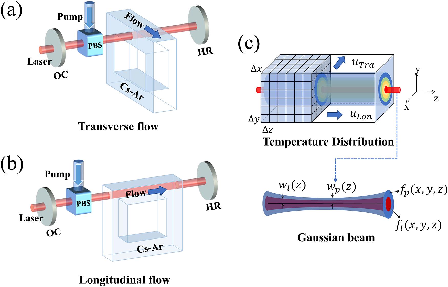
Fig. 1. Sketch of optical systems of XPCsL.

Download full size | View in the Article

Fig. 2. Diagram of energy states in high-power XPCsL system.

Download full size | View in the Article

Fig. 3. Comparison of slope efficiency between experiment^[¹⁹^] and simulation results.

Download full size | View in the Article

Fig. 4. Three-dimensional temperature distribution under different flow directions. The velocity of flow and wall temperature in (a) and (b) are 50 m/s and 473 K.

Download full size | View in the Article

Fig. 5. (a), (b) The temperature distribution in the x–y plane at y = 0 in Figures 4(a) and 4(b). (c), (d) The distribution of

in the x–y plane at y = 0 in Figures 4(a) and 4(b).

Download full size | View in the Article

Fig. 6. Optical-to-optical efficiency and maximum temperature as a function of flow velocity with different pump intensity at T_w = 473 K.

Download full size | View in the Article

Fig. 7. Optical-to-optical efficiency and maximum temperature as a function of flow velocity with different wall temperature at pump intensity of 5 × 10¹⁰ W/m².

Download full size | View in the Article


No.	Process	Cross-section/rate	References
	Thermal associative/dissociative process
1	$\mathrm{Cs}\left({6}^2{S}_{1/2}\right)+ \mathrm{Ar}\rightleftharpoons \mathrm{Cs}\left({X}^2{\varSigma}_{1/2}^{+}\right) \mathrm{Ar}$	${k}_{01},\ {k}_{10}$
			[12]
2	$\mathrm{Cs}\left({B}^2{\varSigma}_{1/2}^{+}\right) \mathrm{Ar}+ \mathrm{Ar}\rightleftharpoons \mathrm{Cs}\left({6}^2{P}_{3/2}\right)+ \mathrm{Ar}$	${k}_{23},\ {k}_{32}$	[12]
	Pumping
3	$\mathrm{Cs}\left({X}^2{\varSigma}_{1/2}^{+}\right) \mathrm{Ar}+h{\nu}_p\to \mathrm{Cs}\left({B}^2{\varSigma}_{1/2}^{+}\right) \mathrm{Ar}$	${P}_{12}$	Equation (9)
	Lasing
4	$\mathrm{Cs}\left({6}^2{P}_{3/2},{6}^2{P}_{1/2}\right)\to \mathrm{Cs}\left({6}^2{S}_{1/2}\right)+h{\nu}_l$	${L}_{30}$	Equation (8)
	Spontaneous emission
5	$\mathrm{Cs}\left({6}^2{P}_{3/2}\right)\to \mathrm{Cs}\left({6}^2{S}_{1/2}\right)+h{\nu}_l$	${A}_{30}$
			[26]
6	$\mathrm{Cs}\left({6}^2{D}_{3/2},{6}^2{D}_{5/2}\right)\to \mathrm{Cs}\left({6}^2{P}_{3/2}\right)+ h\nu$	${A}_{43}$
	Photoexcitation
7	$\mathrm{Cs}\left({6}^2{P}_{3/2},{6}^2{P}_{1/2}\right)+h{\nu}_p\left(h{\nu}_l\right)\to \mathrm{Cs}\left({6}^2{D}_{3/2,5/2},{8}^2{S}_{1/2}\right)$	${Phe}_{34}$	[26]
	Energy pooling
8	$2 \mathrm{Cs}\left({6}^2{P}_{3/2},{6}^2{P}_{1/2}\right)\to \mathrm{Cs}\left({6}^2{D}_{3/2,5/2},{8}^2{S}_{1/2}\right)+ \mathrm{Cs}\left({6}^2{S}_{1/2}\right)$	${Ep}_{34}$	[27]
	Photoionization
9	$\mathrm{Cs}\left({6}^2{D}_{3/2,5/2},{8}^2{S}_{1/2}\right)+h{\nu}_{p,l}\to \mathrm{Cs}^{+}+\mathrm{e}$	${Phi}_{45}$	[27]
	Penning ionization
10	$\mathrm{Cs}\left({6}^2{D}_{3/2,5/2},{8}^2{S}_{1/2}\right)+ \mathrm{Cs}\left({6}^2{P}_{3/2,1/2}\right)\to \mathrm{Cs}^{+}+ \mathrm{Cs}\left({6}^2{S}_{1/2}\right)+\mathrm{e}$	$Pen$	[27]
	Dissociative recombination
11	$\mathrm{Cs}^{+}+ \mathrm{Cs}\left({6}^2{S}_{1/2}\right)+ \mathrm{Cs}\to \mathrm{Cs}_2^{+}+ \mathrm{Cs}$	${R}_1$
12	$\mathrm{Cs}^{+}+ \mathrm{Cs}\left({6}^2{S}_{1/2}\right)+ \mathrm{Ar}\to \mathrm{Cs}_2^{+}+ \mathrm{Ar}$		[26]
13	$\mathrm{Cs}_2^{+}+\mathrm{e}\to \mathrm{Cs}\left({6}^2{D}_{3/2,5/2},{8}^2{S}_{1/2}\right)+ \mathrm{Cs}\left({6}^2{S}_{1/2}\right)$	${R}_2$

Table 1. Kinetic processes in the XPAL system.

View in the Article


Length of cell	Temperature	Pressure of Ar	OC ratio
4 cm	455 K	1270 Torr	0.13

Table 2. Parameters of experiment and simulation.

View in the Article


Parameters	Definition	Value
$L$	Length of the cell	2 cm
$S$	Cross-section of the cell	2 mm$\times$2 mm
${P}_{\mathrm{Ar}}$	Pressure of ethane	1300 Torr
${R}_{\mathrm{oc}}$	OC reflectivity	0.5
${R}_p$	Back mirror reflectivity	0.99
${T}_l$	Single-pass cell window transmission	0.98
${T}_s$	Intra-cavity single-pass loss	0.9
${w}_{0,p}$	Waist of the pump beam	0.5 mm
${w}_{0,l}$	Waist of the laser beam	0.5 mm