• Photonics Research
  • Vol. 5, Issue 3, 176 (2017)
Wei Yan1、2, Yanlong Yang3, Yu Tan2, Xun Chen2, Yang Li2, Junle Qu1、5、*, and Tong Ye2、4、6、*
Author Affiliations
  • 1Key Laboratory of Optoelectronic Devices and Systems of Ministry of Education and Guangdong Province, College of Optoelectronic Engineering, Shenzhen University, Shenzhen 518060, China
  • 2Department of Bioengineering and the COMSET, Clemson University, Clemson, South Carolina 29634, USA
  • 3State Key Laboratory of Transient Optics and Photonics, Xi’an Institute of Optics and Precision Mechanics, Chinese Academy of Science, Xi’an 710119, China
  • 4Department of Regenerative Medicine and Cell Biology, Medical University of South Carolina, Charleston, South Carolina 29425, USA
  • 5e-mail: jlqu@szu.edu.cn
  • 6e-mail: ye7@clemson.edu
  • show less
    DOI: 10.1364/PRJ.5.000176 Cite this Article Set citation alerts
    Wei Yan, Yanlong Yang, Yu Tan, Xun Chen, Yang Li, Junle Qu, Tong Ye. Coherent optical adaptive technique improves the spatial resolution of STED microscopy in thick samples[J]. Photonics Research, 2017, 5(3): 176 Copy Citation Text show less
    Schematic of the COAT-STED microscope. L, lens; GLP, Glan laser polarizer; M, mirrors; DM1 (T: 720–1200 nm, R: 350–720 nm), DM2 (T: 650–800 nm, R: 600–650 nm): dichroic mirrors; GR, glass rod; λ/2, half-wave plate; λ/4, quarter-wave plate; Det, PMT or CCD; SM fiber, single mode fiber; PM fiber, polarization maintaining fiber; MM fiber, multimode fiber.
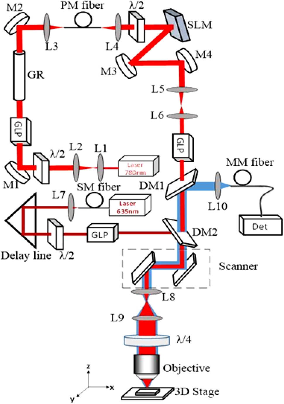
    Fig. 1. Schematic of the COAT-STED microscope. L, lens; GLP, Glan laser polarizer; M, mirrors; DM1 (T: 720–1200 nm, R: 350–720 nm), DM2 (T: 650–800 nm, R: 600–650 nm): dichroic mirrors; GR, glass rod; λ/2, half-wave plate; λ/4, quarter-wave plate; Det, PMT or CCD; SM fiber, single mode fiber; PM fiber, polarization maintaining fiber; MM fiber, multimode fiber.
    (a)–(d) Steps of the COAT phase measurement for directly achieving wavefront correction phase patterns. (e) PSF measured by imaging a GNP mounted on a slide when passing the unmodulated beam though the depletion beam path. (f) PSF of depletion beam after correction. (g) Intensity profiles of the depletion beam before and after correction.
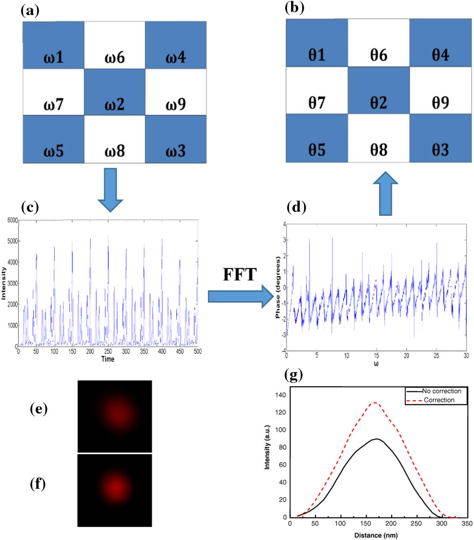
    Fig. 2. (a)–(d) Steps of the COAT phase measurement for directly achieving wavefront correction phase patterns. (e) PSF measured by imaging a GNP mounted on a slide when passing the unmodulated beam though the depletion beam path. (f) PSF of depletion beam after correction. (g) Intensity profiles of the depletion beam before and after correction.
    SLM was configured to provide different phase control segments for aberration correction. (a) Achieved PSFs of no correction and corrected depletion beam with three kinds of phase control segments (correction 1: 1×9 squares, correction 2: 4×9 squares, and correction 3: 9×9 squares). (b) Intensity profiles of the PSFs for no correction, correction 1, correction 2, and correction 3. (c), (d), and (e) Correction phase patterns used for correction 1, 2, and 3, respectively.
    Fig. 3. SLM was configured to provide different phase control segments for aberration correction. (a) Achieved PSFs of no correction and corrected depletion beam with three kinds of phase control segments (correction 1: 1×9 squares, correction 2: 4×9 squares, and correction 3: 9×9 squares). (b) Intensity profiles of the PSFs for no correction, correction 1, correction 2, and correction 3. (c), (d), and (e) Correction phase patterns used for correction 1, 2, and 3, respectively.
    Phantom sample. Middle green region is 5% agarose. Yellow balls are 150 nm GNPs. Red balls are 170 nm FMSs.
    Fig. 4. Phantom sample. Middle green region is 5% agarose. Yellow balls are 150 nm GNPs. Red balls are 170 nm FMSs.
    Correction aberration with COAT (9×9 segments) for the depletion beam path. (a) PSFs of depletion beam with no correction, the system correction, and the full correction. (b) PSF intensity profiles. (c) Phase mask for the system correction. (d) Phase mask for the full correction.
    Fig. 5. Correction aberration with COAT (9×9 segments) for the depletion beam path. (a) PSFs of depletion beam with no correction, the system correction, and the full correction. (b) PSF intensity profiles. (c) Phase mask for the system correction. (d) Phase mask for the full correction.
    Profiles of STED beam PSFs with no correction, system correction, and full correction. Upper: profiles of XY section; bottom: profiles of XZ section.
    Fig. 6. Profiles of STED beam PSFs with no correction, system correction, and full correction. Upper: profiles of XY section; bottom: profiles of XZ section.
    Imaging GNPs overlay beams of no correction and full correction with excitation beam. (a) Overlay beam of no correction. (b) Overlay beam of full correction. (c) PSFs intensity curves of no correction depletion beam, correction depletion beam, and excitation beam.
    Fig. 7. Imaging GNPs overlay beams of no correction and full correction with excitation beam. (a) Overlay beam of no correction. (b) Overlay beam of full correction. (c) PSFs intensity curves of no correction depletion beam, correction depletion beam, and excitation beam.
    (a) Confocal, STED 1 (no correction), STED 2 (system correction), and STED 3 (full correction) images of a single FMS. (b) Normalized intensity profiles of the images.
    Fig. 8. (a) Confocal, STED 1 (no correction), STED 2 (system correction), and STED 3 (full correction) images of a single FMS. (b) Normalized intensity profiles of the images.
    Images of rat heart tissue sample at different depths (7, 19, and 36 μm): The first line are (a) confocal, (b) STED with no correction, and (c) STED with system correction (aberration-corrected STED: AC STED) at 7 μm depth; the second line (d)–(f) are imaging at 19 μm depth; the third line (g)–(i) are imaging at 36 μm depth. The enlarged blue boxed areas are shown in the inset. (j)–(l) Intensity profiles along the blue lines. (m) Final correction phase applied to the SLM.
    Fig. 9. Images of rat heart tissue sample at different depths (7, 19, and 36 μm): The first line are (a) confocal, (b) STED with no correction, and (c) STED with system correction (aberration-corrected STED: AC STED) at 7 μm depth; the second line (d)–(f) are imaging at 19 μm depth; the third line (g)–(i) are imaging at 36 μm depth. The enlarged blue boxed areas are shown in the inset. (j)–(l) Intensity profiles along the blue lines. (m) Final correction phase applied to the SLM.
    Wei Yan, Yanlong Yang, Yu Tan, Xun Chen, Yang Li, Junle Qu, Tong Ye. Coherent optical adaptive technique improves the spatial resolution of STED microscopy in thick samples[J]. Photonics Research, 2017, 5(3): 176
    Download Citation