Optical funnel: broadband and uniform compression of electromagnetic fields to an air neck

Fei Sun; Yichao Liu; Yibiao Yang

doi:10.1364/PRJ.432030

Abstract

An optical funnel, which performs as a passive electromagnetic compressor, can guide electromagnetic waves from a wide inlet to a narrow outlet without reflectance/scattering and squeeze electromagnetic fields uniformly to an air neck. In this study, an optical funnel is designed by precisely filling subwavelength ceramic blocks with a gradient refractive index inside a tapered waveguide. The gradient refractive index is designed by transformation optics, which is isotropic and all above unit, thus exhibiting a broadband feature. Due to the mechanism of impedance matching over the whole funnel, extremely low reflectance/scattering and stable enhancement of fields can be achieved. The field enhancement factor in different regions of the funnel (e.g., in the air neck) can be flexibly designed just by modifying the funnel-width ratios.

1. INTRODUCTION

The enhancement of electromagnetic (EM) fields has wide applications in various fields, such as nano antenna [1,2], EM sensing [3,4], solar cells [5,6], and biosensing [7,8]. Especially in the field of weak optical/EM signal detection, a compact passive EM compressor, which can compress EM fields in free space to obtain a large uniform and stable enhancement factor for a broad frequency band, is highly required. Surface plasmon polaritons (SPPs) are one way to enhance the weak electric fields, e.g., surface-enhanced Raman spectroscopy (SERS) [9] uses SPPs to enhance the weak electric fields in Raman scattering [10,11]. In addition to SERS, SPPs are also used in other cases for EM field enhancement in optical detection and sensing, e.g., plasmon-enhanced nanopillar photodetectors operating in the near-infrared spectral regime [12] and plasmon-enhanced fluorescence [13]. Electric field enhancement by SPPs has poor local uniformity due to the protruding nanoparticles or artificial structures on the surface and is usually confined in narrow bandwidth due to the resonance nature of the SPPs. With the development of metamaterials, several kinds of novel methods to enhance the EM fields have been proposed, e.g., concentrators [14,15] or singular structures [16] based on transformation optics, epsilon-near-zero materials [17], mu-near-zero materials [18], and plasma antenna arrays [19]. Transformation optics-based EM concentrators squeeze EM fields into a region filled by materials with high permittivity or permeability, which is not convenient for subsequent detection. Singular structures or arrays usually confine light to the region with sharp tips, which leads to nonuniform position-sensitive enhancement of the fields and seriously affects stability/robustness for the detection of weak fields, especially for the sensing system. Materials with near-zero parameters usually suffer from a narrow band and material loss. Therefore, there is still no effective method to achieve broadband uniform EM field enhancement in an air region.

In this study, an optical funnel [see Fig. 1(a)], which can compress the EM field from its wide inlet to its narrow outlet without reflectance, is designed to solve the above problem. The enhanced EM fields can be achieved in the air neck of the optical funnel [see Fig. 1(a)], which is more convenient for subsequent system integration (e.g., optical sensors). The EM field enhancement factor can be designed by changing the funnel-width ratios, i.e., $w_{1} / w_{2}$ for the electric fields and $w_{1} / w_{3}$ for the magnetic fields [ $w_{1}$ , $w_{2}$ , and $w_{3}$ are the width of the inlet, the outlet, and the neck; see Fig. 1(a)], which provides more flexibility and adjustability in different applications. The proposed optical funnel can be widely used as the passive pre-amplification structure of various optical systems to enhance EM fields.

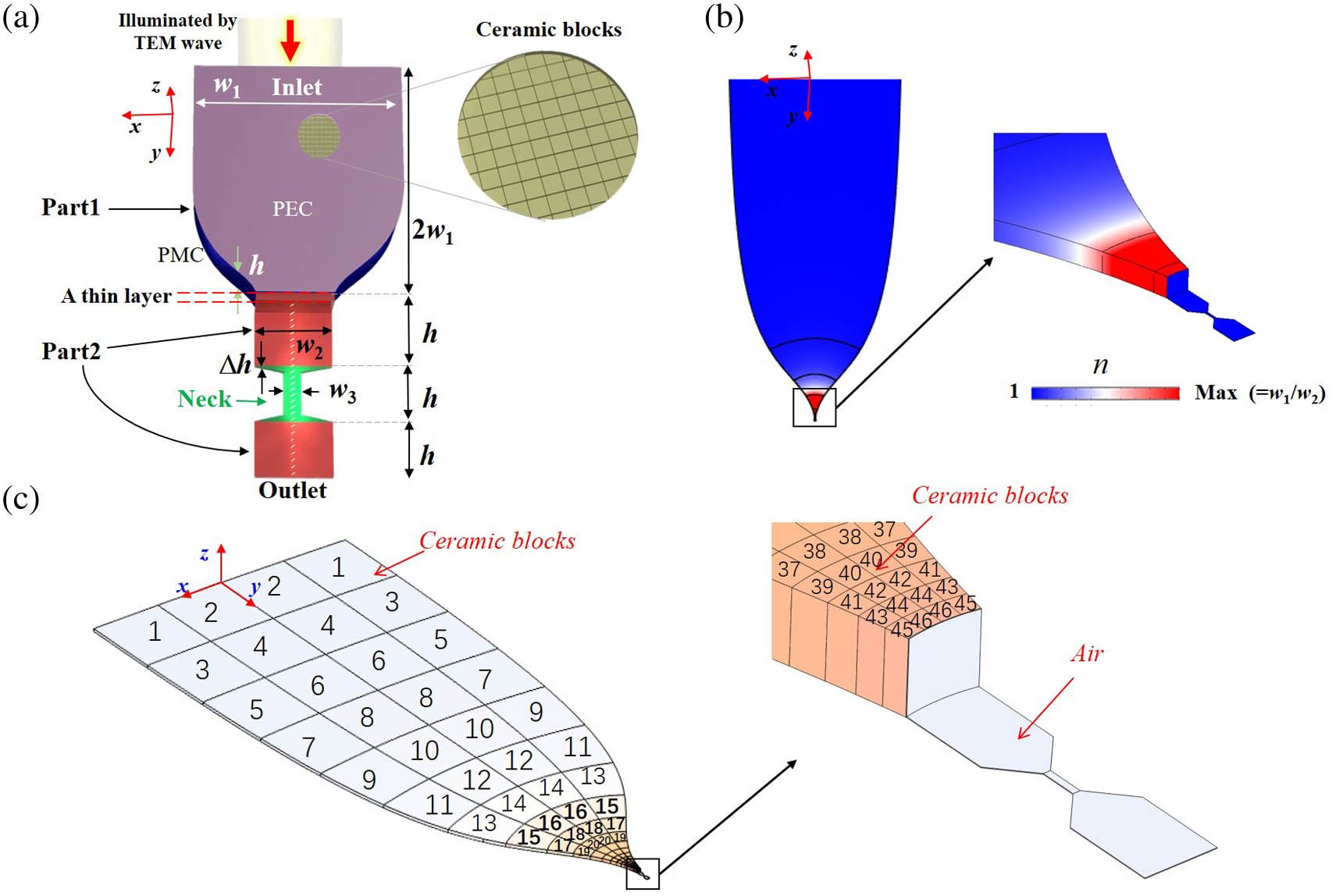
$(a) Structural diagram of the optical funnel. PEC (colored pink) and PMC (colored blue) are used as the top/bottom and side boundaries of the whole funnel, respectively. To show the internal structure of the funnel more clearly, the PEC and PMC on part 2 (colored red) and the neck (colored green) are not drawn. (b) Refractive index distribution of the whole structure. (c) An implementable structure of the designed optical funnel by filling ceramic blocks with different permittivity (indicated by different colors and numbers) or air inside the waveguide, where w1=2λ0/3, w2=0.01w1, w3=0.001w1, h=0.01w1, Δh=0.01h, and the working wavelength λ0=3 m.$

Figure 1.(a) Structural diagram of the optical funnel. PEC (colored pink) and PMC (colored blue) are used as the top/bottom and side boundaries of the whole funnel, respectively. To show the internal structure of the funnel more clearly, the PEC and PMC on part 2 (colored red) and the neck (colored green) are not drawn. (b) Refractive index distribution of the whole structure. (c) An implementable structure of the designed optical funnel by filling ceramic blocks with different permittivity (indicated by different colors and numbers) or air inside the waveguide, where $w_{1} = 2 λ_{0} / 3$ , $w_{2} = 0.01 w_{1}$ , $w_{3} = 0.001 w_{1}$ , $h = 0.01 w_{1}$ , $Δ h = 0.01 h$ , and the working wavelength $λ_{0} = 3 m$ .

2. MATERIALS AND METHODS

The structural diagram of the proposed optical funnel is shown in Fig. 1(a), which is a tapered EM waveguide and consists of two parts. The waveguide is covered by perfect electric conductors (PECs) at the top and bottom, and covered by perfect magnetic conductors (PMCs) at the side boundaries. Part 1 is the front part of the funnel, which performs as a waveguide adaptor filled with dielectrics of the gradient refractive index designed by transformation optics. Part 1 has a fixed height of $h$ and varied width from the funnel’s inlet $w_{1}$ to $w_{2}$ . The length of part 1 is designed as $2 w_{1}$ , which can ensure that the refractive index at the funnel’s inlet is equal to 1. Part 2 is the back part of the funnel, which is an air-filled waveguide (designed by transmission line theory) and contains an air neck inside. The funnel’s inlet and outlet are in the front of part 1 and in the end of part 2, respectively.

Sign up for Photonics Research TOC. Get the latest issue of Photonics Research delivered right to you！Sign up now

The function of part 1 is to compress the incident fields from its wider funnel’s inlet to its narrower port without reflection, which achieves the first level magnetic field enhancement. The thin layer between part 1 and part 2 can guide the compressed EM fields smoothly to the height-reduced part 2 (filled with air) without reflection, i.e., achieving the electric field enhancement. The funnel’s neck can achieve the secondary enhancement of only magnetic fields by reducing the neck width. If only electric fields need to be enhanced, the funnel’s neck can be removed. In the funnel, EM fields are gradually compressed along the axis of the optical funnel (the $y$ axis) from the inlet in part 1 to the outlet in part 2 and achieve a uniform enhanced EM field at the air neck/outlet (see Visualization 1 and Visualization 2 for the transient fields of $E_{z}$ and $H_{x}$ ).

For part 1, transformation optics [20,21] is used to design the gradient refractive index inside the tapered waveguide, which has matched impedance and ensures that the absorption and reflection/scattering are sufficiently small. By using a conformal transformation, the front part of the funnel (part 1) can be designed with varied width and gradient refractive index [see Fig. 1(b)], which can squeeze the EM fields smoothly to its narrower port without reflection. The distribution of the relative permittivity (relative permeability = 1) in the tapered waveguide can be written as (see Appendix A for detail) $ε (x, y) = 1 + \frac{w_{1}^{4}}{16 {(x^{2} + y^{2})}^{2}} + \frac{w_{1}^{2} (x^{2} - y^{2})}{2 {(x^{2} + y^{2})}^{2}},$ (1)which ranges from one (funnel’s inlet) to the maximum value of ${(w_{1} / w_{2})}^{2}$ (determined by the electric field enhancement factor $A_{E}$ ). The gradient refractive index in part 1 of the designed optical funnel can be realized by filling ceramic blocks with different permittivity inside the waveguide; see the inset of Fig. 1(a). The size of each ceramic block is about one-fifth of the local wavelength, i.e., $λ / 5$ , which satisfies the requirement of the effective medium theory [22]. For the back part of the funnel (part 2 and the air neck), transmission line theory can be used to design a proper size and filling material. Since the final EM-enhanced region (i.e., the funnel’s outlet/neck) should be air, the size of the waveguide in part 2 needs to be precisely designed by transmission line theory (to satisfy that the impedance is always the same as that of the waveguide in part 1). In our design, the length (the $y$ direction), width (the $x$ direction), and height (the $z$ direction) of the air-filled waveguide in part 2 are designed as $3 h$ , $w_{2}$ , and $Δ h = h w_{2} / w_{1}$ (see Appendix B for detail). Although part 1 and part 2 have the same characteristic impedance, the large difference between their heights leads to the boundary effect, which will cause severe reflections. A thin subwavelength air layer (with height $h$ in the $z$ direction and length $Δ h = λ_{0} / 15,000$ in the $y$ direction) connecting part 1 and part 2 can well eliminate the boundary effect and ensure low reflectance (see Appendix B). The funnel’s neck is embedded in part 2 with a further reduced width $w_{3}$ , which will not introduce obvious scattering due to the quasi-static character of the fields in part 2. The EM fields are transmitted from the front part to the back part of the designed funnel with the same characteristic impedance but different height. Since the impedance is matched along the axis of the optical funnel, no reflection appears, which further ensures a considerable enhancement of EM fields.

As an example of the above design, an optical funnel with $w_{2} = 0.01 w_{1}$ can be realized by filling 92 ceramic blocks with different permittivities in part 1 [see Fig. 1(c)]. The permittivity of the 46 ceramic blocks [23] (only half of the blocks are given due to symmetry) in a frequency range from 1 MHz to 0.1 GHz is listed in Table 1. Note the boundary of the ceramic blocks is not necessarily straight, i.e., the boundary shape of the ceramic blocks can be chosen freely. Orthogonal curves are used as the boundary of the ceramic blocks, which can better fit the curved boundaries of the funnel. Note the filling materials can be any dielectric blocks as long as they satisfy the designed permittivity distribution in Eq. (1). Ceramic blocks with different doping concentrations [23] can precisely meet the requirement of the permittivity distribution in Table 1 from 1 MHz to 0.1 GHz and are therefore used in the design.Table 1.

Permittivity of the Ceramic Blocks^a

Number	1	2	3	4	5	6	7	8	9	10	11	12
$ε_{r}$	1.1	1.1	1.2	1.2	1.2	1.3	1.3	1.4	1.6	1.7	2.0	2.3
Number	13	14	15	16	17	18	19	20	21	22	23	24
$ε_{r}$	3.3	3.7	6.8	7.3	16	16	36.0	34.5	74.4	70.8	142	136
Number	25	26	27	28	29	30	31	32	33	34	35	36
$ε_{r}$	253	243	424	409	674	654	1027	1001	1510	1477	2150	2110
Number	37	38	39	40	41	42	43	44	45	46
$ε_{r}$	2982	2933	4040	3982	5362	5295	6991	6914	8971	8883

The sequence numbers correspond to the numbers in Fig. 1(c).

The electric and magnetic fields enhancement factors ( $A_{E}$ and $A_{H}$ ) are defined as the ratio of the electric/magnetic fields’ amplitude in different regions of the funnel to the incident electric/magnetic fields’ amplitude, which are also related to the width in different regions of the funnel when the incident wave is the transverse EM (TEM) wave. In the air neck, the field enhancement factors can be theoretically derived as (see Appendix C) ${\begin{matrix} A_{E} = \frac{E^{(3)}}{E^{(0)}} = \frac{w_{1}}{w_{2}} \\ A_{H} = \frac{H^{(3)}}{H^{(0)}} = \frac{w_{1}}{w_{3}} \end{matrix},$ (2)where the superscript (3) represents the EM fields inside the funnel’s neck, and the superscript (0) represents incident EM fields at the inlet; see the corresponding regions in Fig. 2(a). Regions (1) and (2) represent part 1 and part 2 of the funnel, respectively.

Figure 2.Simulated results. (a) Amplitudes of electric fields and magnetic fields distributions inside the funnel when a TEM wave of unit amplitude is illuminated onto the inlet of the designed optical funnel. (b) Electric fields (red) and magnetic fields (blue) enhancement factor along the axis of the optical funnel ( $x = 0$ ), where $w_{1} = 2 / 3 λ_{0}$ , $w_{2} = 0.01 w_{1}$ , $w_{3} = 0.1 w_{2}$ , $h = 0.01 w_{1}$ , and $Δ h = 0.01 h$ . (1), (2), and (3) represent the corresponding regions in (a).

The amplitudes of the electric and magnetic fields inside the designed optical funnel are shown in Fig. 2(a). The corresponding enhancement factors along the funnel in different regions are shown in Fig. 2(b), which shows that the funnel can squeeze EM waves gradually from the inlet to the funnel’s neck/outlet. The simulated enhancement factors [the red and blue solid lines for $A_{E}$ and $A_{H}$ , respectively, in Fig. 2(b)] in region (3) fit well with theoretical predictions in Eq. (2) [the yellow and green dashed lines for $A_{E}$ and $A_{H}$ , respectively, in Fig. 2(b)] with funnel-width ratios $w_{1} / w_{2} = 100$ and $w_{1} / w_{3} = 1000$ . Note nonlinear axes are used in Fig. 3(b) for a clear view of the enhancement in different regions. The three regions have different enhancement effects on electric and magnetic fields. Region (1) has no enhancement effect on electric fields, while regions (2) and (3) can enhance electric fields uniformly. Both regions (1) and (3) can enhance the magnetic fields gradually (more details can be found in Appendix C).

Figure 3.Average value (dots; left $y$ axis), standard deviations (error bars; left $y$ axis), and uniformity (blue squares and red diamonds; right $y$ axis) of the (a) electric fields and (b) magnetic fields with varied funnel width in the funnel’s neck (at 0.1 GHz). Average value (dots; left $y$ axis), standard deviations (error bars; left $y$ axis), and uniformity (red diamonds; right $y$ axis) of the (c) electric fields and (d) magnetic fields in the funnel’s neck with varied frequency (with funnel-width ratios $w_{1} / w_{2} = 100$ and $w_{1} / w_{3} = 1000$ ).

3. RESULTS AND DISCUSSION

A. Uniformity of the Enhanced EM Fields

The designed optical funnel can create uniform enhanced EM fields inside the funnel’s air neck [see Fig. 2(a)]. To numerically verify the uniformity of the enhanced EM fields with varied structure sizes and frequencies, the uniformity can be quantitatively defined as the coefficient of variation of the fields (smaller coefficient of variation means better uniformity): ${\begin{matrix} C_{E} = \frac{σ_{E}}{E_{avg}} \\ C_{H} = \frac{σ_{H}}{H_{avg}} \end{matrix},$ (3)where $E_{avg} = \frac{\iint E d s}{S}$ and $H_{avg} = \frac{\iint H d s}{S}$ are the average amplitude ( $x − y$ plane) of the electric fields and magnetic fields, $S$ denotes the cross-sectional area in $x − y$ plane of the funnel’s neck, and $E$ and $H$ denote the amplitude of the electric fields and magnetic fields. $σ_{E} = \sqrt{[\iint {(E - E_{avg})}^{2} d s] / S}$ and $σ_{H} = \sqrt{[\iint {(H - H_{avg})}^{2} d s] / S}$ are the standard deviations of the electric fields and magnetic fields. The uniformity of the electric fields and magnetic fields varies accordingly with the funnel-width ratios (i.e., $w_{1} / w_{2}$ and $w_{2} / w_{3}$ ), which are shown in Figs. 3(a) and 3(b). The error bar represents the standard deviations of the fields, and the dots represent the average values of the fields (on the left $y$ axis). The uniformity $C_{E}$ and $C_{H}$ (blue squares and red diamonds) are represented in Figs. 3(a) and 3(b) on the right y axis. It shows that the uniformity of the electric fields is better for larger $w_{1} / w_{2}$ and smaller $w_{2} / w_{3}$ , while the uniformity of the magnetic fields is independent on $w_{1} / w_{2}$ and gets better for larger $w_{2} / w_{3}$ . The coefficient of variation of both the electric fields and magnetic fields still keeps a small value ( $C_{E} < 0.1$ and $C_{H} < 0.1$ ) for all these funnel-width ratios, i.e., the enhanced EM fields inside the funnel’s air neck have good uniformity with varied width of the funnel. The uniformity is also good in a broad frequency range (from 1 MHz to 0.1 GHz), which is shown in Figs. 3(e) and 3(f). The simulated results show that the designed funnel has high uniformity of the enhancement factor in the funnel’s air neck for varied funnel width in a broad working frequency band.

B. Enhancement Factor with Varied Funnel Width

The electric and magnetic field enhancement factors [ $A_{E}$ and $A_{H}$ in Eq. (2)] are completed as determined by the geometrical size of the optical funnel (i.e., funnel-width ratios $w_{1} / w_{2}$ and $w_{2} / w_{3}$ ). Therefore, various enhancement factors for electric and magnetic fields can be obtained by choosing corresponding funnel-width ratios (i.e., $w_{1} / w_{2}$ and $w_{2} / w_{3}$ ) of the designed optical funnel. The numerical simulation results in Figs. 4(a) and 4(b) show the electric and magnetic fields enhancement factors in the air neck for different funnel-width ratios, which coincide with the theoretical calculation results in Figs. 4(c) and 4(d). The working wavelength is the same as the one in Fig. 1. Figure 4 and Eq. (2) provide convenient instructions on how to pick suitable funnel widths for achieving a pre-designed enhancement factor. The magnetic fields have larger enhancement factors than electric fields due to the secondary enhancement in the funnel’s neck (see Fig. 4), which means the designed funnel is very suitable to create large magnetic fields from weak background fields.

Figure 4.(a), (b) Numerical simulation and (c), (d) theoretical calculation results for the electric and magnetic fields enhancement factors in the funnel’s air neck, respectively, when the funnel-width ratios ( $w_{1} / w_{2}$ and $w_{2} / w_{3}$ ) of the designed optical funnel vary.

C. Bandwidth Analysis

Since ceramic blocks in Table 1 with weak dispersion in a wide frequency band can exactly meet the required permittivity of the optical funnel in Eq. (1), the designed optical funnel can achieve a broadband EM fields concentrating effect. Numerical simulations in Fig. 5 show the electric/magnetic fields enhancement factors in the air neck of the designed funnel, which shows the relative stable enhancement effect for both electric fields ( $A_{E} ⩾ 100$ ) and magnetic fields ( $A_{H} ⩾ 990$ ) within a frequency range from 1 MHz to 0.1 GHz and verifies broadband features of the funnel. If the working frequency further increases, the enhancement factor will drop rapidly as the effective medium theory cannot be satisfied, and, at the same time, high-order modes will be excited, which also increase reflectance. The optical funnel can also work in higher frequency bands with proper filling materials (e.g., metamaterials with high refractive index in the terahertz [24], infrared [25,26], and optical ranges [27]).

Figure 5.Simulated results: the relation between the working frequency and the electric/magnetic fields enhancement factors $A_{E}$ (red) and $A_{H}$ (blue) in the air neck of the designed funnel with fixed funnel-width ratios $w_{1} / w_{2} = 100$ and $w_{1} / w_{3} = 1000$ .

4. CONCLUSION

Although the light funnel in this study has a similar shape to the nonimaging light concentrators (NLCs) [28 –31], which are widely used in solar cells for light concentration, there are many differences between the optical funnel in this study and the NLCs. The NLCs are designed by nonimaging optics [28], which can be realized by silicon (no gradient media are required). The optical funnel in this study is designed by transformation optics [20,21], which needs well-designed gradient distribution of the refractive index. The enhancement obtained by NLC arrays is caused by the efficient occupation of Mie modes, which is motivated by its unique geometry [29]. However, from the perspective of transformation optics, the enhancement obtained by our optical funnel is due to the compression of spatial geometry. The geometric sizes of the NLCs are usually on the subwavelength order, while the overall size of our funnel can be larger than the wavelength. Compared with NLCs, the optical funnel in this study has a lower reflectivity and can achieve a uniform enhancement in the air region, whose enhancement factor is directly determined by the geometric ratio in Eq. (2). However, the optical funnel in this study requires complex material parameter distribution and is valid for only one polarization. Therefore, the designed optical funnel in this study is different from the NLCs in terms of theoretical design, material realization, working characteristics, geometric size, etc.

For a physical realization, three kinds of materials should be used to build an optical funnel, i.e., PEC, PMC, and dielectric blocks. In the designed frequency range (i.e., 1 MHz to 0.1 GHz), dielectric blocks have been well designed by using ceramic blocks [23] [see Fig. 1(c)]. The PEC and PMC can be realized by metal sheets [32] and artificial structures/surfaces [33,34], respectively. For higher frequency bands, dielectric blocks can be realized by metamaterials [24 –27]. The PEC and PMC can be approximately realized by some metasurfaces [35] and artificial structures [36].

In conclusion, an optical funnel, which can smoothly compress incident EM fields from the inlet to the outlet/neck along the funnel axis and achieve a broadband uniform EM field enhancement at the outlet/neck, is designed by precise placement of weakly dispersive ceramic blocks with a gradient refractive index. The electric/magnetic fields enhancement factors in different regions of the funnel can be flexibly pre-designed by adjusting the funnel-width ratios. Large and stable enhancement of both electric and magnetic fields (e.g., over 100 times) can be achieved in the air neck of the funnel over a broad frequency range from 1 MHz to 0.1 GHz. The designed passive funnel can be used as a passive pre-amplification structure for weak optical/EM field enhancement and detection, e.g., SERS, optical sensing, EM field concentration.

APPENDIX A: DESIGN OF PART 1

z

Figure 6.(a) In the reference space, 2D structural correspondence between the rectangular waveguides and (b) the optical funnel in the real space, respectively, based on the coordinate transformation in Eq. (4).

w_{2}

APPENDIX B: DESIGN OF PART 2

Z = \sqrt{\frac{μ}{ε}} \frac{h}{w}

APPENDIX C: ENHANCEMENT FACTORS IN DIFFERENT REGIONS

0 < y < y_{1}

Figure 7.Funnel 2D view ( $x − y$ plane) from Fig. 1(a). Different $y$ coordinates indicate different locations in the funnel: $y = y_{1}$ represents the end of part 1; $y = y_{2}$ represents the end of the thin layer; $y = y_{3}$ represents the end of part 2 (the upper part); and $y = y_{4}$ represents the end of part 3.

y_{1} < y < y_{2}

y_{2} < y < y_{3}

y_{3} < y < y_{4}

Using Eqs. (C1)-(C3), the theoretical values for the field enhancements at the funnel’s neck in Eq. (2) can be derived.

References

[1] J. Xia, J. Tang, F. Bao, Y. Sun, M. Fang, G. Cao, J. Evans, S. He. Turning a hot spot into a cold spot: polarization-controlled Fano-shaped local-field responses probed by a quantum dot. Light Sci. Appl., 9, 166(2020).

[2] H. Linnenbank, Y. Grynko, J. Förstner, S. Linden. Second harmonic generation spectroscopy on hybrid plasmonic/dielectric nanoantennas. Light Sci. Appl., 5, e16013(2016).

[3] O. Stranik, H. McEvoy, C. McDonagh, B. MacCraith. Plasmonic enhancement of fluorescence for sensor applications. Sens. Actuators B, 107, 148-153(2005).

[4] M. I. Stockman. Nanoplasmonic sensing and detection. Science, 348, 287-288(2015).

[5] C. Hägglund, M. Zäch, G. Petersson, B. Kasemo. Electromagnetic coupling of light into a silicon solar cell by nanodisk plasmons. Appl. Phys. Lett., 92, 053110(2008).

[6] L. Etgar. Semiconductor nanocrystals as light harvesters in solar cells. Materials, 6, 445-459(2013).

[7] Y. Yanase, T. Hiragun, S. Kaneko, H. J. Gould, M. W. Greaves, M. Hide. Detection of refractive index changes in individual living cells by means of surface plasmon resonance imaging. Biosens. Bioelectron., 26, 674-681(2010).

[8] V. Chabot, Y. Miron, M. Grandbois, P. G. Charette. Long range surface plasmon resonance for increased sensitivity in living cell biosensing through greater probing depth. Sens. Actuators B, 174, 94-101(2012).

[9] P. L. Stiles, J. A. Dieringer, N. C. Shah, R. P. Van Duyne. Surface-enhanced Raman spectroscopy. Annu. Rev. Anal. Chem., 1, 601-626(2008).

[10] C. Matricardi, C. Hanske, J. L. Garcia-Pomar, J. Langer, A. Mihi, L. M. Liz-Marzan. Gold nanoparticle plasmonic superlattices as surface-enhanced Raman spectroscopy substrates. ACS Nano, 12, 8531-8539(2018).

[11] K. N. Kanipe, P. P. Chidester, G. D. Stucky, M. Moskovits. Large format surface-enhanced Raman spectroscopy substrate optimized for enhancement and uniformity. ACS Nano, 10, 7566-7571(2016).

[12] P. Senanayake, C.-H. Hung, J. Shapiro, A. Lin, B. Liang, B. S. Williams, D. Huffaker. Surface plasmon-enhanced nanopillar photodetectors. Nano Lett., 11, 5279-5283(2011).

[13] J. Dong, Z. Zhang, H. Zheng, M. Sun. Recent progress on plasmon-enhanced fluorescence. Nanophotonics, 4, 472-490(2015).

[14] M. Rahm, D. Schurig, D. A. Roberts, S. A. Cummer, D. R. Smith, J. B. Pendry. Design of electromagnetic cloaks and concentrators using form-invariant coordinate transformations of Maxwell’s equations. Photon. Nanostr. Fundam. Appl., 6, 87-95(2008).

[15] P.-F. Zhao, L. Xu, G.-X. Cai, N. Liu, H.-Y. Chen. A feasible approach to field concentrators of arbitrary shapes. Front. Phys., 13, 134205(2018).

[16] Y. Luo, R. Zhao, A. I. Fernandez-Dominguez, S. A. Maier, J. B. Pendry. Harvesting light with transformation optics. Sci. China Inf. Sci., 56, 1-13(2013).

[17] M. G. Silveirinha, N. Engheta. Theory of supercoupling, squeezing wave energy, and field confinement in narrow channels and tight bends using ε near-zero metamaterials. Phys. Rev. B, 76, 245109(2007).

[18] Y. Jin, P. Zhang, S. He. Squeezing electromagnetic energy with a dielectric split ring inside a permeability-near-zero metamaterial. Phys. Rev. B, 81, 085117(2010).

[19] W. Shi, B. Yuan, J. Mao, C. Wang. Enhancement of electromagnetic energy by plasma antenna. Nano Energy, 76, 105053(2020).

[20] J. B. Pendry, D. Schurig, D. R. Smith. Controlling electromagnetic fields. Science, 312, 1780-1782(2006).

[21] U. Leonhardt. Optical conformal mapping. Science, 312, 1777-1780(2006).

[22] M. Wang, N. Pan. Predictions of effective physical properties of complex multiphase materials. Mater. Sci. Eng. R Rep., 63, 1-30(2008).

[23] Y. Li, W. Li, G. Du, N. Chen. Low temperature preparation of CaCu₃Ti₄O₁₂ ceramics with high permittivity and low dielectric loss. Ceram. Int., 43, 9178-9183(2017).

[24] M. Choi, S. H. Lee, Y. Kim, S. B. Kang, J. Shin, M. H. Kwak, K.-Y. Kang, Y.-H. Lee, N. Park, B. Min. A terahertz metamaterial with unnaturally high refractive index. Nature, 470, 369-373(2011).

[25] H. Krishnamoorthy, G. Adamo, J. Yin, V. Savinov, N. Zheludev, C. Soci. Infrared dielectric metamaterials from high refractive index chalcogenides. Nat. Commun., 11, 1692(2020).

[26] J.-T. Shen, P. B. Catrysse, S. Fan. Mechanism for designing metallic metamaterials with a high index of refraction. Phys. Rev. Lett., 94, 197401(2005).

[27] J. Y. Kim, H. Kim, B. H. Kim, T. Chang, J. Lim, H. M. Jin, J. H. Mun, Y. J. Choi, K. Chung, J. Shin, S. Fan, S. O. Kim. Highly tunable refractive index visible-light metasurface from block copolymer self-assembly. Nat. Commun., 7, 12911(2016).

[28] R. Winston, J. C. Miñano, P. G. Benitez. Nonimaging Optics(2005).

[29] G. Marko, A. Prajapati, G. Shalev. Subwavelength nonimaging light concentrators for the harvesting of the solar radiation. Nano Energy, 61, 275-283(2019).

[30] A. Prajapati, Y. Nissan, T. Gabay, G. Shalev. Broadband absorption of the solar radiation with surface arrays of subwavelength light funnels. Nano Energy, 54, 447-452(2018).

[31] A. Prajapati, A. Chauhan, D. Keizman, G. Shalev. Approaching the Yablonovitch limit with free-floating arrays of subwavelength trumpet non-imaging light concentrators driven by extraordinary low transmission. Nanoscale, 11, 3681-3688(2019).

[32] G. D. Bai, F. Yang, W. X. Jiang, Z. L. Mei, T. J. Cui. Realization of a broadband electromagnetic gateway at microwave frequencies. Appl. Phys. Lett., 107, 153503(2015).

[33] M. L. Chen, L. J. Jiang, W. E. Sha. Artificial perfect electric conductor-perfect magnetic conductor anisotropic metasurface for generating orbital angular momentum of microwave with nearly perfect conversion efficiency. J. Appl. Phys., 119, 064506(2016).

[34] A. Erentok, P. L. Luljak, R. W. Ziolkowski. Characterization of a volumetric metamaterial realization of an artificial magnetic conductor for antenna applications. IEEE Trans. Antennas Propag., 53, 160-172(2005).

[35] C. Liu, G. Gan, X. Cui. Visible perfect reflectors realized with all-dielectric metasurface. Opt. Commun., 402, 226-230(2017).

[36] C. Valagiannopoulos, A. Tukiainen, T. Aho, T. Niemi, M. Guina, S. Tretyakov, C. Simovski. Perfect magnetic mirror and simple perfect absorber in the visible spectrum. Phys. Rev. B, 91, 115305(2015).

[37] L. Xu, H. Chen. Conformal transformation optics. Nat. Photonics, 9, 15-23(2015).

[38] R. E. Collin. Field Theory of Guided Waves, 5(1990).