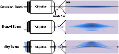
Fig. 1. Configuration of the Gaussian, Bessel, and Airy beams with the same light-sheet FOV.

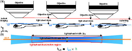
Fig. 2. Schematic of Gaussian beam light-sheet z-stacking imaging. (a) z-stacking imaging by moving light-sheet and objective. (b) Illumination region and system DOF under the large FOV imaging.

Fig. 3. Flowchart of 3D image deblurring processing.

Fig. 4. Schematic of our light-sheet microscope setup. Galvo z and Galvo y are used to scan the beam along the z-axis and y-axis, respectively. IO and DO are the illumination and detection objectives, respectively.

Fig. 5. Comparisons of different deconvolution methods. (a) Simulated 3D image (ground truth) in the x−y, x−z, and y−z sections, and three colored subregions enlarged for a detailed observation at the bottom. (b) Blurred 3D image after forward 3D convolution and Gaussian and Poisson mixed noise addition. (c)–(f) Four reconstruction results using the 2D RL method, the 3D Wiener method, the 3D RL method, and our 3D method, respectively. The R value in the title represents the correlation coefficient of the 3D distribution between the ground truth and each deblurred image.

Fig. 6. Contrast comparison of 3D deconvolution methods for imaging a 6 μm hollow fluorescence microsphere. (a) Middle x−y sections of the observed 3D image and three reconstructed images from the 3D RL method, the 3D Wiener method, and our 3D method. Scale bar: 3 μm. (b) Four normalized profiles corresponding to the colored dashed lines in (a).

Fig. 7. Comparison of 2D and 3D deconvolution for imaging the rhombencephalon activity of 7 dpf Tg (elavl3:GCaMP6s) zebrafish larva, recorded by 1328 (x)×1328 (y)×81 (z) voxels. (a) Selected x−y, x−z, and y−z sections of the raw image (observed image) and our image (our 3D method). Scale bar: 50 μm. (b) The corresponding cyan, yellow, and magenta subregions in (a) were enlarged for a comparison between 2D (2D RL method) and 3D deconvolution (our 3D method).

Fig. 8. Comparison of different 3D deconvolution methods for imaging the rhombencephalon structure of 6 dpf Tg (elavl3:EGFP) zebrafish larva, recorded by 1928 (x)×1928 (y)×81 (z) voxels. (a) Selected x−y, x−z, and y−z sections of the raw image (observed image) and our image (our 3D method). Scale bar: 50 μm. (b) The corresponding cyan, yellow, and magenta subregions in (a) were enlarged for a comparison of three reconstruction results (3D Wiener method, 3D RL method, and our 3D method). (c) Power spectral distributions (8×8×1 binning). Three z-stacking movies corresponding to three reconstruction results are provided in Visualization 1, Visualization 2, and Visualization 3.

Fig. 9. SNR comparison of the 3D deconvolution methods for imaging the mesencephalon activity of 7 dpf Tg (elavl3:H2B-GCaMP6s) zebrafish larva, recorded by 1448 (x)×1448 (y)×81 (z) voxels. (a) The 32nd x−y section of the raw image (observed image) and our image (our 3D method). The corresponding cyan subregion of the x−y section on the left was enlarged for a comparison of three reconstruction results (3D Wiener method, 3D RL method, and our 3D method). Scale bar: 50 μm. (b) The 724th x−z section of the observed image (3D Wiener method, 3D RL method, and our 3D method), where the magenta and yellow subregions were enlarged for a clear observation. Scale bar: 50 μm. (c) Normalized distribution of the yellow profiles labeled in (a), where the blue bars in (c) mark all the regions of the suspected neuron boundary by manual identification. (d) Average modified signal-to-noise ratio (MSNR) of the fluorescence peaks along lines across the neuron from images reconstructed with the 3D Wiener method, the 3D RL method, and our 3D method (n=9). Centerline: medians. Limits: 75% and 25%. Whiskers: maximum and minimum. Three z-stacking movies corresponding to three reconstruction results are provided in Visualization 4, Visualization 5, and Visualization 6.

Fig. 10. Destriping results for imaging the rhombencephalon structure of 6 dpf Tg (elavl3:EGFP) zebrafish larva, recorded by 1928 (x)×1928 (y) pixels. (a) Image after using the destriping algorithm. Scale bar: 50 μm. (b) The corresponding subregions before and after destriping in (a) were enlarged for a comparison. (c) Two normalized profiles corresponding to the colored dashed lines in (b).