1LMAM, School of Mathematical Sciences, Peking University, Beijing 100871, China
2State Key Laboratory of Membrane Biology, Beijing Key Laboratory of Cardiometabolic Molecular Medicine, Institute of Molecular Medicine, Peking University, Beijing 100871, China
3Center for Bioinformatics, National Laboratory of Protein Engineering and Plant Genetic Engineering, School of Life Sciences, Peking University, Beijing 100871, China
4School of Software and Microelectronics, Peking University, Beijing 100871, China
5Beijing Advanced Innovation Center for Imaging Theory and Technology, Capital Normal University, Beijing 100871, China
Due to its ability of optical sectioning and low phototoxicity, -stacking light-sheet microscopy has been the tool of choice for in vivo imaging of the zebrafish brain. To image the zebrafish brain with a large field of view, the thickness of the Gaussian beam inevitably becomes several times greater than the system depth of field (DOF), where the fluorescence distributions outside the DOF will also be collected, blurring the image. In this paper, we propose a 3D deblurring method, aiming to redistribute the measured intensity of each pixel in a light-sheet image to in situ voxels by 3D deconvolution. By introducing a Hessian regularization term to maintain the continuity of the neuron distribution and using a modified stripe-removal algorithm, the reconstructed -stack images exhibit high contrast and a high signal-to-noise ratio. These performance characteristics can facilitate subsequent processing, such as 3D neuron registration, segmentation, and recognition.
1. INTRODUCTION
Fluorescence microscopy (FM) can provide both in vitro and in vivo imaging of biological tissues as well as their functional dynamics, which is observable with high spatial and temporal resolution [1–3]. Moreover, benefiting from the various choices of fluorescent indicators for neuronal activities, FM has been widely used for in vivo brain imaging [4–9]. However, because a large number of neurons are spread in the brain region [10], brain imaging must record neuronal activities with a large field of view (FOV) simultaneously [11–13]. For example, three-dimensional imaging of the zebrafish brain should cover a volume of μμμwith subneuron resolution.
Different from confocal [14], spinning disk confocal [15], multiphoton [16], and light-field [17] FMs, selective plane illumination microscopy [18–20] (also called light-sheet microscopy) has recently emerged as the preferable method for volumetric imaging of the zebrafish brain. Based on -scanning light-sheet illumination, the brain region can be excited slice-by-slice, and these side-sliced fluorescent images are built into the volumetric stack. This form of microscopy, originally designed for highly efficient optical sectioning, can effectively enhance the image contrast and reduce the phototoxicity in deep tissues [20].
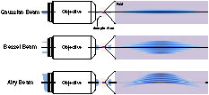
Figure 1.Configuration of the Gaussian, Bessel, and Airy beams with the same light-sheet FOV.
According to Gaussian beam propagation [14], the relationship between the light-sheet thickness () and light-sheet nominal width () is given as where is the wavelength in vacuum, is the refractive index of the medium on the object side, is the waist radius of the Gaussian beam, and is the Rayleigh length of the Gaussian beam. As illustrated, imaging with a wider FOV uses a thicker Gaussian beam.
Sign up for Photonics Research TOC. Get the latest issue of Photonics Research delivered right to you!Sign up now
Generally, thin light-sheet -stacking images have desired optical sectioning and -axis spatial resolution and do not require 3D deconvolution, since the thickness of light-sheet illumination is very close to the system depth of field (DOF) [20]. However, for zebrafish brain-wide imaging, the light sheet is thicker, where the fluorescence distributions outside the DOF will also be collected, blurring the image. Therefore, we resort to 3D deconvolution to redistribute the measured intensity from the -stack images. Meanwhile, the nonuniform illumination of a Gaussian beam will produce an additional difference in each light-sheet image. In addition, melanogenesis tissues located at the surface of the fish head locally and significantly absorb the excitation energy, which also leads to dark stripes in the light-sheet image [24].
To address the abovementioned problems in zebrafish larva brain-wide imaging, we implement a thick Gaussian beam light-sheet microscope and expand the width of the light sheet to greater than 300 μm, which makes the thickness of the light sheet more than 8 μm, nearly 9.6-fold the system DOF. In this paper, we first derive an approximated 3D convolution forward model for thick light-sheet -stacking imaging and propose a 3D deblurring method by introducing a Hessian regularization term to maintain the continuity of the neuron distribution. Employing this 3D reconstruction algorithm and a modified stripe-removal algorithm, the reconstructed -stack images can exhibit high contrast and a high signal-to-noise ratio (SNR).
This paper is organized as follows. Section 2 introduces the forward model and 3D deblurring algorithm. Section 3 presents our experimental setup and preparation. Sections 4 and 5 present the results of both a numerical simulation and imaging experiments on fluorescent beads and a zebrafish larvae brain. Section 6 concludes and discusses the paper.
2. THEORY
A. Forward Model
Figure 2.Schematic of Gaussian beam light-sheet -stacking imaging. (a) -stacking imaging by moving light-sheet and objective. (b) Illumination region and system DOF under the large FOV imaging.
Assume that the illumination distribution is uniform in the plane and symmetric with respect to the -axis, i.e., . Assume that the system 3D point spread function (PSF) is space-invariant in the brain area. The imaging forward model of thick Gaussian beam light-sheet microscopy can be approximated as follows (see Appendix A): where is the true volumetric image, is the 2D blurred image when the illumination and detection are located at the plane, is the overall 3D PSF affected by the illumination, and .
B. 3D Reconstruction Algorithm
Here, we define a loss function as the sum of the fidelity term and Hessian regularization term, which is also popular in other imaging modalities [25,26]. The Hessian regularization term is from a priori knowledge of zebrafish brain (see Section 6). The fidelity term constrains the imaging forward model by using the mean square error, and the Hessian regularization term constrains the continuity of the neuron distribution. Such a loss function can be written as where is the penalty parameter of the fidelity term. The Hessian regularization is defined as where and are the penalty parameters of continuity along the x−y plane and -axis, respectively. The second-order partial derivatives of in different directions are abbreviated as .
In this paper, we use the alternating direction method of multipliers (ADMM) [27] to solve this loss function based on its fast convergence performance in an -regularized optimization problem. The key of the algorithm is to decouple the and portions from the loss function [28]. Hence, we rewrite Eq. (3) by introducing auxiliary variables and using the augmented Lagrangian methods (see Appendix B): where are the auxiliary and dual variables, is the step size, and is the iteration counter.
Consequently, the framework of the ADMM algorithm is presented in Algorithm 1.
Evaluation Indicators of Different 3D Images in Fig. 5
PSNR
SNR
SSIM
Blurred Image
16.60
1.99
0.044
0.62
2D RL
16.30
1.69
0.072
0.57
3D Wiener
16.83
2.22
0.149
0.64
3D RL
16.56
1.95
0.158
0.68
Our 3D Method
18.46
3.86
0.179
0.84
Table Infomation Is Not Enable
C. Full Procedure
In real experiments, light-sheet images are corrupted with photon shot noise and camera readout noise. We use the side window filtering (SWF) technique [29] to eliminate the mixed Poisson–Gaussian noise in the fluorescence image. In contrast to conventional local window-based filtering methods, the SWF method aligns the edges and/or corners of the window with the pixels being processed, which better preserves the image boundaries during the denoising process.
Furthermore, nonneuron melanogenesis tissues located at the surface of the fish head can absorb the excitation energy dramatically, which results in dark stripes along the excitation path. The widely used wavelet-FFT algorithm can be used to remove the stripe artifacts [30] but at cost price of deteriorating the image in regions devoid of stripes. Therefore, we introduce a prelocation method based on the output of the wavelet-FFT algorithm. Specifically, the positions and widths of all stripes are determined from the difference map between the original image and the wavelet-FFT processed image. Only the stripe areas in the original image will be multiplied with an adaptive Gaussian stripe function to correct for the artifacts. This modified algorithm can avoid information loss outside the stripe areas and provide consistent contrast across different regions of the image.
Figure 3.Flowchart of 3D image deblurring processing.
Figure 4.Schematic of our light-sheet microscope setup. Galvo and Galvo are used to scan the beam along the -axis and -axis, respectively. IO and DO are the illumination and detection objectives, respectively.
All larval zebrafish (elavl3:H2B-GCaMP6s, elavl3:GCaMP6s, and elavl3:EGFP) were raised in E3 embryo medium according to the standard protocol under 28.5°C. 0.2 mmol/L 1-phenyl-2-thiourea was added to the embryo medium to inhibit melanogenesis and allow optical imaging of the brain region. In our light-sheet imaging experiment, a 5–7 day post fertilization (dpf) zebrafish will be anesthetized before being embedded in a 1.5% low-melting agarose cylinder with a diameter of 1 mm and immersed in E3 medium. The brain area was electrically aligned to the center of the detection FOV being in good posture for -stacking imaging.
The 3D PSF could be calibrated with sparse fluorescent beads statically embedded in the agarose cylinder or calculated by using the ImageJ plugin PSF generator and using the system parameters. The light-sheet illumination distribution could only be captured from the system utilizing imaging with a high-density fluorescent bead mixed medium. As shown in Eq. (2), the overall 3D PSF is given by the product of and . After the imaging experiments, the results showed that the calculated PSF is better than the calibrated PSF during the reconstruction iteration (see Section 6).
The experiments are implemented on an HP Z6 Workstation (Intel Xeon Gold 6128 CPU @ 3.40 GHz × 24), the graphics card model is GeForce RTX 2080 Ti, and the operating system is Ubuntu 19.04. The 3D deconvolution algorithm is implemented using MATLAB R2019b.
4. SIMULATION
Figure 5.Comparisons of different deconvolution methods. (a) Simulated 3D image (ground truth) in the x−y, x−z, and y−z sections, and three colored subregions enlarged for a detailed observation at the bottom. (b) Blurred 3D image after forward 3D convolution and Gaussian and Poisson mixed noise addition. (c)–(f) Four reconstruction results using the 2D RL method, the 3D Wiener method, the 3D RL method, and our 3D method, respectively. The value in the title represents the correlation coefficient of the 3D distribution between the ground truth and each deblurred image.
Then, the ground truth was convolved with the overall 3D PSF function according to Eq. (2) followed by the introduction of Gaussian and Poisson mixed noise to generate a blurred 3D image stack [Fig. 5(b)]. These images were deconvolved with four deconvolution methods, the 2D Richardson–Lucy (RL) method, the 3D RL method [31,32], the 3D Wiener method [33], and our 3D method (also called the Hessian method) (see Section 2) [Figs. 5(c)–5(f)]. RL and Wiener are popular deconvolution algorithms for fluorescence microscopy images [34]. Of course, many software packages, such as DeconvolutionLab2 [35], also include the 3D RL and 3D Wiener algorithms and so on, but considering the consistency of the computing platform and the stability of performance, we choose the code provided by the MATLAB toolbox. We calculated four evaluation indicators, including the peak signal-to-noise ratio (PSNR) [36], SNR [33], structural similarity (SSIM) index [37], and correlation coefficient (R) [38] between the blurred image and four deblurred 3D image stacks, as shown in Table 1. The higher the indicator value, the closer the reconstructed image is to the real situation. Therefore, from this calculation, it is obvious that our method can recover more correct high-frequency components with much less noise.
5. IMAGING EXPERIMENTS
Figure 6.Contrast comparison of 3D deconvolution methods for imaging a 6 μm hollow fluorescence microsphere. (a) Middle x−y sections of the observed 3D image and three reconstructed images from the 3D RL method, the 3D Wiener method, and our 3D method. Scale bar: 3 μm. (b) Four normalized profiles corresponding to the colored dashed lines in (a).
There are three typical zebrafish lines frequently used for in vivo brain imaging, Tg (elavl3:EGFP), Tg (elavl3:GCaMP6s), and Tg (elavl3:H2B-GCaMP6s), which have neuronal-specific expression of GFP, the calcium indicator GCaMP6s localized in the cytoplasm of neurons, and the calcium indicator GCaMP6s localized in the nuclei of neurons, respectively.
Figure 7.Comparison of 2D and 3D deconvolution for imaging the rhombencephalon activity of 7 dpf Tg (elavl3:GCaMP6s) zebrafish larva, recorded by voxels. (a) Selected x−y, x−z, and y−z sections of the raw image (observed image) and our image (our 3D method). Scale bar: 50 μm. (b) The corresponding cyan, yellow, and magenta subregions in (a) were enlarged for a comparison between 2D (2D RL method) and 3D deconvolution (our 3D method).
Figure 8.Comparison of different 3D deconvolution methods for imaging the rhombencephalon structure of 6 dpf Tg (elavl3:EGFP) zebrafish larva, recorded by voxels. (a) Selected x−y, x−z, and y−z sections of the raw image (observed image) and our image (our 3D method). Scale bar: 50 μm. (b) The corresponding cyan, yellow, and magenta subregions in (a) were enlarged for a comparison of three reconstruction results (3D Wiener method, 3D RL method, and our 3D method). (c) Power spectral distributions ( binning). Three -stacking movies corresponding to three reconstruction results are provided in Visualization 1, Visualization 2, and Visualization 3.
Figure 9.SNR comparison of the 3D deconvolution methods for imaging the mesencephalon activity of 7 dpf Tg (elavl3:H2B-GCaMP6s) zebrafish larva, recorded by voxels. (a) The 32nd x−y section of the raw image (observed image) and our image (our 3D method). The corresponding cyan subregion of the x−y section on the left was enlarged for a comparison of three reconstruction results (3D Wiener method, 3D RL method, and our 3D method). Scale bar: 50 μm. (b) The 724th x−z section of the observed image (3D Wiener method, 3D RL method, and our 3D method), where the magenta and yellow subregions were enlarged for a clear observation. Scale bar: 50 μm. (c) Normalized distribution of the yellow profiles labeled in (a), where the blue bars in (c) mark all the regions of the suspected neuron boundary by manual identification. (d) Average modified signal-to-noise ratio (MSNR) of the fluorescence peaks along lines across the neuron from images reconstructed with the 3D Wiener method, the 3D RL method, and our 3D method (). Centerline: medians. Limits: 75% and 25%. Whiskers: maximum and minimum. Three -stacking movies corresponding to three reconstruction results are provided in Visualization 4, Visualization 5, and Visualization 6.
Figure 10.Destriping results for imaging the rhombencephalon structure of 6 dpf Tg (elavl3:EGFP) zebrafish larva, recorded by pixels. (a) Image after using the destriping algorithm. Scale bar: 50 μm. (b) The corresponding subregions before and after destriping in (a) were enlarged for a comparison. (c) Two normalized profiles corresponding to the colored dashed lines in (b).
For zebrafish larva brain-wide imaging, light-sheet illumination is required to cover a large FOV and possess concentrated energy in the focal plane. For this purpose, we implemented a thick Gaussian beam light-sheet microscope and expanded the width of the light sheet to more than 300 μm, making the thickness of the light sheet more than 8 μm, nearly 9.6-fold the system DOF. Our 3D deblurring method has been proposed to redistribute the measured intensity of each pixel in the light-sheet image to in situ voxels by 3D deconvolution. By introducing a Hessian regularization term to maintain the continuity of the neuron distribution and using a modified stripe-removal algorithm, the reconstructed -stack images exhibit high contrast and a high SNR. These performance characteristics can facilitate subsequent processing, such as 3D neuron segmentation and recognition.
Comparing Fig. 5(c) with Fig. 5(f) in the simulation section, it has been verified that 3D deconvolution is more effective than 2D deconvolution for thick light-sheet imaging. In addition, comparing the different 3D deconvolution methods, especially referring to the reconstructed movies, our 3D deblurring method (see Fig. 3), including stripe-removal postprocessing, has been validated.
Here, we present some discussions concerning the deblurring methods and imaging settings. System.Xml.XmlElementSystem.Xml.XmlElementSystem.Xml.XmlElementSystem.Xml.XmlElementSystem.Xml.XmlElementSystem.Xml.XmlElementSystem.Xml.XmlElementSystem.Xml.XmlElement
APPENDIX A
The formation of light-sheet images is related to 3D PSF and illumination distribution. A generalized 3D light-sheet imaging forward model is presented in this section.
The coordinate in our system is shown in Fig.?4. We assume that the observed biological sample is located in a rectangular region . The light sheet is formed by rapidly scanning the Gaussian beam along the -axis, and it is easy to have In addition, the light sheet is symmetrical along the -axis, i.e., Let the area satisfy , , where the 3D PSF is invariant in the subarea , and the light-sheet illumination distribution is uniform in the subarea , i.e., In this case, the light-sheet images are obtained by this model: In our system, we consider that the illumination distribution is uniform and the 3D PSF is invariant in the FOV of zebrafish brain. Therefore, the light-sheet image is the convolution of the overall PSF and the observed biological sample.
APPENDIX B
In this section, 3D deconvolution with Hessian regularization solved by the ADMM algorithm is presented. We rewrite Eq.?(3) as where subject to According to augmented Lagrangian and the method of multipliers, we compute the following update steps for each ADMM iteration: Alternately solve the joint optimization of each variable as follows. The -minimization step is expressed as and the -minimization step is expressed as and the dual variables , are solved by where is a step size and is the iteration counter.
The -minimization involves solving a minimum Euclidean norm problem. And is solved by where fft is the fast Fourier transform, and ifft is the inverse fast Fourier transform. is the second-order partial derivative operator in the direction, i.e., , and , , , , , and are defined similarly.
The -minimization involves solving a closed-form solution by using subdifferential calculus. And the auxiliary variables , are solved by
[27] S. Boyd, N. Parikh, E. Chu, B. Peleato, J. Eckstein. Distributed Optimization and Statistical Learning via the Alternating Direction Method of Multipliers(2011).
[43] M. Temerinac-Ott, O. Ronneberger, R. Nitschke, W. Driever, H. Burkhardt. Spatially-variant Lucy-Richardson deconvolution for multiview fusion of microscopical 3D images. 2011 IEEE International Symposium on Biomedical Imaging: From Nano to Macro, 899-904(2011).