• Photonics Research
  • Vol. 5, Issue 2, 64 (2017)
Weixing Shu1、4、*, Xiaohui Ling2、3, Xiquan Fu1, Yachao Liu2, Yougang Ke2, and Hailu Luo2、5、*
Author Affiliations
  • 1College of Computer Science and Electronic Engineering, Hunan University, Changsha 410082, China
  • 2Laboratory for Spin Photonics, School of Physics and Electronics, Hunan University, Changsha 410082, China
  • 3College of Physics and Electronic Engineering, Hengyang Normal University, Hengyang 421002, China
  • 4e-mail: wxshu@hnu.edu.cn.
  • 5e-mail: hailuluo@hnu.edu.cn.
  • show less
    DOI: 10.1364/PRJ.5.000064 Cite this Article Set citation alerts
    Weixing Shu, Xiaohui Ling, Xiquan Fu, Yachao Liu, Yougang Ke, Hailu Luo. Polarization evolution of vector beams generated by q-plates[J]. Photonics Research, 2017, 5(2): 64 Copy Citation Text show less
    Polarization distributions of vector fields generated by q-plates for different incident waves. The first column shows the theoretical results for an incident plane wave, while the others show an incident Gaussian beam. The four rows correspond to incidences of right, left, and right circular and linear polarizations (σ=+1,−1,+1,0), respectively. The q-plates used have q=1 and α0=π/4 in the upper two rows and q=1 and α0=0 in the other rows. The dimension for all images is w0×w0, where w0=1.75 mm.
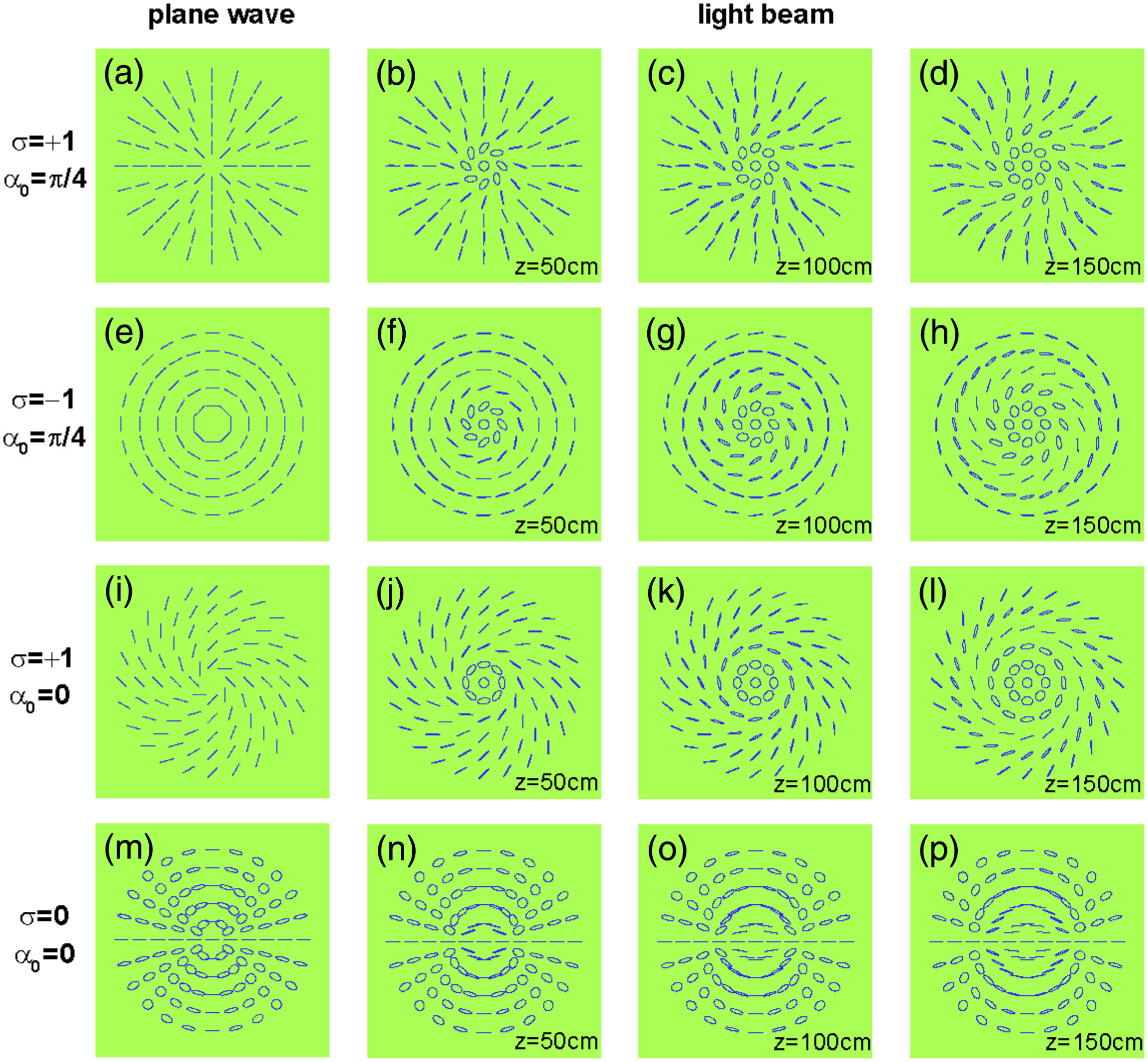
    Fig. 1. Polarization distributions of vector fields generated by q-plates for different incident waves. The first column shows the theoretical results for an incident plane wave, while the others show an incident Gaussian beam. The four rows correspond to incidences of right, left, and right circular and linear polarizations (σ=+1,1,+1,0), respectively. The q-plates used have q=1 and α0=π/4 in the upper two rows and q=1 and α0=0 in the other rows. The dimension for all images is w0×w0, where w0=1.75  mm.
    Polarization evolution on the Poincaré sphere. (a) For the vector vortex beam in Fig. 1(j), the polarization states along a radial direction (from r=0 to ∞ for a given θ) evolve from the north pole to the south pole. For the vector field in Fig. 1(i), the states in a radial direction correspond to a single point that does not change with propagation. (b) For the VB in Fig. 1(n), the polarization states on circles with different radii around the beam center evolve along different 8-shaped curves. Here, r0=0.3 mm is the radius of the first circle in Fig. 1. For the vector field in Fig. 1(m), the states on all circles evolve along the same 8-shaped curve.
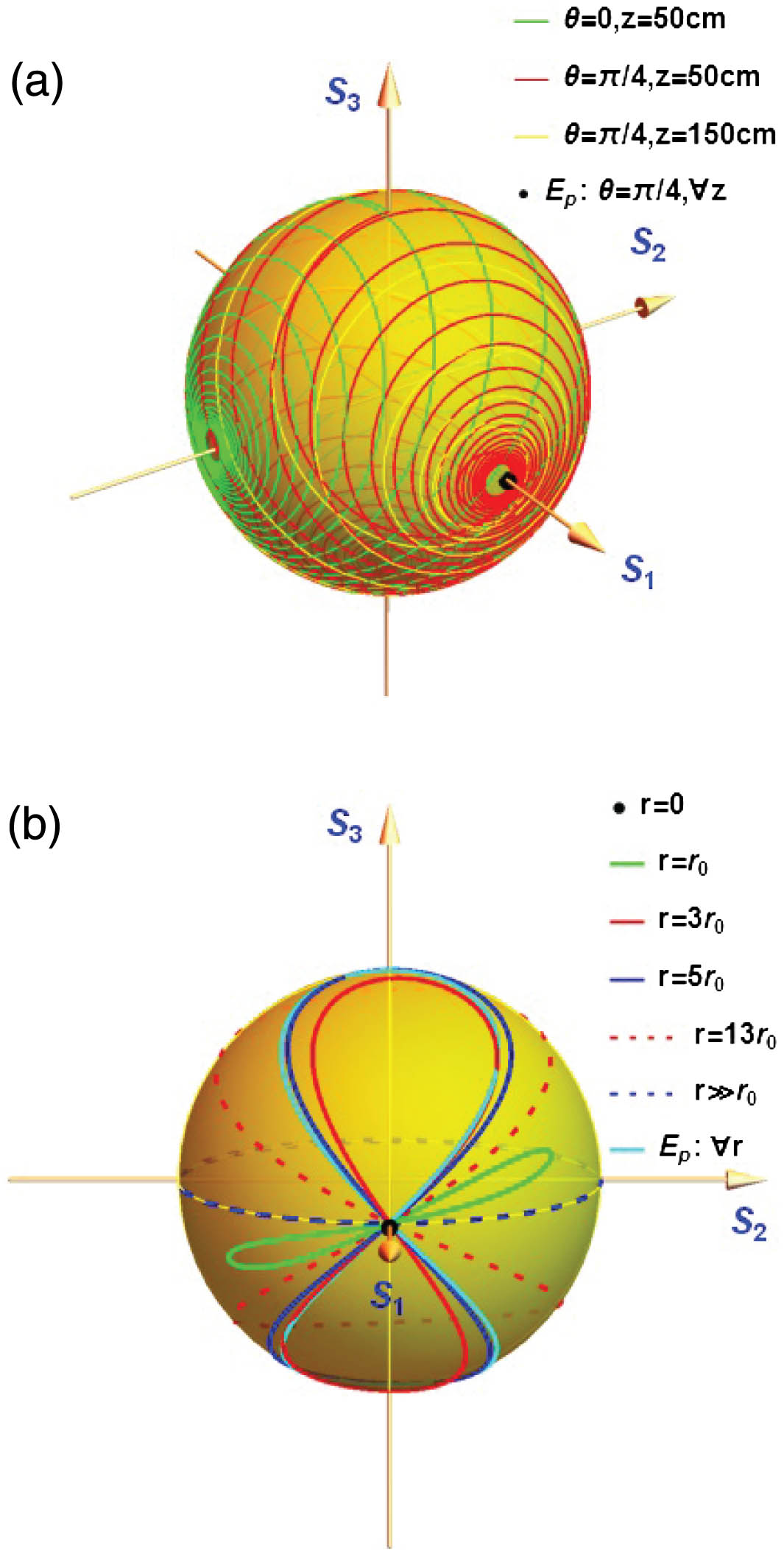
    Fig. 2. Polarization evolution on the Poincaré sphere. (a) For the vector vortex beam in Fig. 1(j), the polarization states along a radial direction (from r=0 to for a given θ) evolve from the north pole to the south pole. For the vector field in Fig. 1(i), the states in a radial direction correspond to a single point that does not change with propagation. (b) For the VB in Fig. 1(n), the polarization states on circles with different radii around the beam center evolve along different 8-shaped curves. Here, r0=0.3  mm is the radius of the first circle in Fig. 1. For the vector field in Fig. 1(m), the states on all circles evolve along the same 8-shaped curve.
    Schematic of experimental setup to generate VBs. The inset is a schematic drawing of the q-plate with q=1 and α0=π/4. White short lines denote the orientations of local optical axes.
    Fig. 3. Schematic of experimental setup to generate VBs. The inset is a schematic drawing of the q-plate with q=1 and α0=π/4. White short lines denote the orientations of local optical axes.
    Intensities and polarizations measured on the transverse plane z=50 cm. The top and bottom rows result from the incidence of right and left circularly polarized Gaussian beams, respectively. The left and right columns are the theoretical and experimental results, respectively. Here the q-plate with q=1 and α0=π/4 is used. The size for all images is 2.4 mm×2.3 mm.
    Fig. 4. Intensities and polarizations measured on the transverse plane z=50  cm. The top and bottom rows result from the incidence of right and left circularly polarized Gaussian beams, respectively. The left and right columns are the theoretical and experimental results, respectively. Here the q-plate with q=1 and α0=π/4 is used. The size for all images is 2.4  mm×2.3  mm.
    For the radially polarized beam in Fig. 4(a), (a) is the intensity through a linear polarizer with the transmission axis indicated by the arrow; (b) and (c) are the intensities of the left and right circularly polarized components, respectively. The bottom row shows the experimental results corresponding to the top one.
    Fig. 5. For the radially polarized beam in Fig. 4(a), (a) is the intensity through a linear polarizer with the transmission axis indicated by the arrow; (b) and (c) are the intensities of the left and right circularly polarized components, respectively. The bottom row shows the experimental results corresponding to the top one.
    For the azimuthally polarized beam Fig. 4(c), (a) is the intensity through a linear polarizer with the transmission axis indicated by the arrow; (b) and (c) are the intensities of the left and right circularly polarized components, respectively. In the bottom row are the experimental results corresponding to the top one.
    Fig. 6. For the azimuthally polarized beam Fig. 4(c), (a) is the intensity through a linear polarizer with the transmission axis indicated by the arrow; (b) and (c) are the intensities of the left and right circularly polarized components, respectively. In the bottom row are the experimental results corresponding to the top one.
    Transverse intensities and polarizations for a spirally polarized VB at different propagation distances. The top, middle, and bottom rows correspond to z=50, 100, and 150 cm, respectively. The left and right columns are the theoretical and experimental results, respectively. Here the incident Gaussian beam is right circularly polarized and the q-plate with q=1 and α0=0 is used. The size for all images is 2.4 mm×2.3 mm.
    Fig. 7. Transverse intensities and polarizations for a spirally polarized VB at different propagation distances. The top, middle, and bottom rows correspond to z=50, 100, and 150 cm, respectively. The left and right columns are the theoretical and experimental results, respectively. Here the incident Gaussian beam is right circularly polarized and the q-plate with q=1 and α0=0 is used. The size for all images is 2.4  mm×2.3  mm.
    (a) Theoretical and (b) experimental results of the radial intensity distributions for the spirally polarized beam in Fig. 7. The intensities are normalized by the center intensity of the incident Gaussian beam. (c) Theoretical and (d) experimental results of the radial intensity distributions for the spirally polarized beam and its two circular polarization components measured at z=50 cm. On top are the local polarization states. (e) is the evolution of polarization states along a radial line (0≤r≤2.5 mm and θ=π/4).
    Fig. 8. (a) Theoretical and (b) experimental results of the radial intensity distributions for the spirally polarized beam in Fig. 7. The intensities are normalized by the center intensity of the incident Gaussian beam. (c) Theoretical and (d) experimental results of the radial intensity distributions for the spirally polarized beam and its two circular polarization components measured at z=50  cm. On top are the local polarization states. (e) is the evolution of polarization states along a radial line (0r2.5  mm and θ=π/4).
    Transverse intensity and polarization distribution for the VB generated by a linearly polarized Gaussian beam passing through a q-plate. (a) Theoretical results calculated by Eq. (16) and (b) experimental results measured at z=50 cm. Here, the q-plate with q=1 and α0=0 is used. The size for all images is 2.4 mm×2.3 mm.
    Fig. 9. Transverse intensity and polarization distribution for the VB generated by a linearly polarized Gaussian beam passing through a q-plate. (a) Theoretical results calculated by Eq. (16) and (b) experimental results measured at z=50  cm. Here, the q-plate with q=1 and α0=0 is used. The size for all images is 2.4  mm×2.3  mm.
    (a) and (b) are the transverse intensities for two circularly polarized components, respectively, and (c) the Stokes parameter S3, corresponding to the VB in Fig. 9. The second rows are correspondent experimental results.
    Fig. 10. (a) and (b) are the transverse intensities for two circularly polarized components, respectively, and (c) the Stokes parameter S3, corresponding to the VB in Fig. 9. The second rows are correspondent experimental results.
    Polarization evolution on the Poincaré sphere. Shown are the theoretical and experimental results for the third string of polarization states (with a radius r=3r0) on the beam cross section in Fig. 9.
    Fig. 11. Polarization evolution on the Poincaré sphere. Shown are the theoretical and experimental results for the third string of polarization states (with a radius r=3r0) on the beam cross section in Fig. 9.
    Weixing Shu, Xiaohui Ling, Xiquan Fu, Yachao Liu, Yougang Ke, Hailu Luo. Polarization evolution of vector beams generated by q-plates[J]. Photonics Research, 2017, 5(2): 64
    Download Citation