Polarization evolution of vector beams generated by q-plates

Weixing Shu; Xiaohui Ling; Xiquan Fu; Yachao Liu; Yougang Ke; Hailu Luo

doi:10.1364/PRJ.5.000064

Abstract

The polarization evolution of vector beams (VBs) generated by

q

-plates is investigated theoretically and experimentally. An analytical model is developed for the VB created by a general quarter-wave

q

-plate based on vector diffraction theory. It is found that the polarization distribution of VBs varies with position and the value

q

. In particular, for the incidence of circular polarization, the exit vector vortex beam has polarization states that cover the whole surface of the Poincaré sphere, thereby constituting a full Poincaré beam. For the incidence of linear polarization, the VB is not cylindrical but specularly symmetric, and exhibits an azimuthal spin splitting. These results are in sharp contrast with those derived by the commonly used model, i.e., regarding the incident light as a plane wave. By implementing

q

-plates with dielectric metasurfaces, further experiments validate the theoretical results.

Keywords

Berry''s phase Diffraction theory Form birefringence Metamaterials Optical vortices Polarization

1. INTRODUCTION

Vector beams (VBs) with inhomogeneous polarization have lately attracted much attention ^[1]. Different from the common homogeneously polarized beams, VBs have unique optical properties owing to their inherent symmetry. For example, a radially polarized light beam, when tightly focused, can have a strong longitudinal and nonpropagating electric field ^[2], resulting in a sharper focus than a homogeneously polarized beam ^[3]. This result leads to significant enhancements in the interaction between light and material ^[4] and in the microscope resolution ^[5]. In addition, an azimuthally polarized beam can be highly focused into a hollow dark spot ^[3,6]. Due to their distinguished properties, VBs have found applications in a variety of realms ranging from classical to quantum optics. In classical optics, VBs have be used in optical trapping ^[7], optical microfabrication ^[8], ultra-sensitive metrology ^[9], high-resolution imaging ^[5,10], optical data storage ^[11], polarization encryption ^[12], and optical communications ^[13]. In the quantum regime, VBs have been applied to create hybrid entangled states exploiting the polarization and the spatial degrees of freedom to realize quantum communications ^[14,15].

Motivated by these applications, various methods for generating VBs have been proposed ^[1], which may be divided into two classes. One is the intracavity generation technique involving the coherent summation of two orthogonally polarized modes inside either the laser resonator ^[16,17] or optical fibers that are also cylindrically symmetric resonators ^[18,19]. The other method is the extracavity generation that includes the interferometric combination of orthogonally polarized beams ^[20–27] and the direct conversion of uniformly polarized light using polarization-sensitive optical elements. Such optical elements can be implemented by segmented birefringent crystals ^[28,29], subwavelength diffractive gratings ^[30–32], and twisted liquid crystals ^[33,34]. These devices are characterized by singular optic axis distributions with topological charge $q$ and are usually called $q$ -plates ^[33].

The VBs generated by the direct conversion method are often analyzed by regarding the light beam as a plane wave in the literature. Actually, this simplified model can conveniently account for the vector polarization generated by the commonly used half-wave $q$ -plates ^[35–38]. For these $q$ -plates there occurs a complete conversion between the two circular polarization components of the incident light ^[33], and thus the polarization of the combined VB is the same as that obtained by replacing the beam with a plane wave and does not change upon propagation ^[39].

Sign up for Photonics Research TOC. Get the latest issue of Photonics Research delivered right to you！Sign up now

However, for a $q$ -plate with an arbitrary phase retardation, this plane wave model may not hold true. For a general $q$ -plate, an incomplete cross-polarization conversion may occur ^[40,41]. The converted light interferes with the residual beam, and, consequently, the generated VB possesses a hybrid polarization that may change during propagation ^[32] and may even lead to a spin Hall effect of light ^[40–42]. Actually, it was shown recently that a superposition of a vortex beam and a Gaussian beam with opposite circular polarizations, similar to the two components generated by the $q$ -plate, results in a polarization distribution on a transverse plane covering the whole Poincaré sphere ^[43,44]. Therefore it is not only necessary but interesting to consider the practical dimensions of VBs. However, except for the approximate plane-wave model, there is still not an accurate model to describe the polarization of VB created by a general $q$ -plate.

In this paper, we take into account the beam dimensions to investigate the polarization of VBs generated with $q$ -plates. First, an explicit form of VB beyond a quarter-wave $q$ -plate is established based on vector diffraction theory. Second, this model is applied to investigate the polarization evolution of VBs. It is found that the transverse distribution of polarizations of VBs vary with position and the value $q$ . In particular, for the incidence of circular polarization, the exit vector vortex beam has polarization states that can cover the whole Poincaré sphere and then belongs to full Poincaré beams. For the incidence of linear polarization, the VB is not cylindrical but specularly symmetric, and exhibits an azimuthal splitting of spin. These results are entirely different from those derived by the plane wave model for the incident light. Applying our model, the underlying mechanisms to the polarization and intensity profiles of the VBs are revealed. By implementing $q$ -plates with dielectric metasurfaces, further experiments are made to verify the theoretical results.

2. THEORETICAL FORMULATION

Let us consider a homogeneous elliptically polarized light normally incident on a wave plate. This polarization can be expressed in terms of its polar angle $ϑ$ and azimuthal angle $ϕ$ on the Poincaré sphere ^[44,45]: where $E_{0} (x, y)$ is the amplitude, and $| + ⟩ = (\hat{x} + i \hat{y}) / \sqrt{2}$ and $| - ⟩ = (\hat{x} - i \hat{y}) / \sqrt{2}$ represent the right and left circular polarization states, respectively.

We choose a uniaxial wave plate for which the transmission coefficients are $t_{s}$ and $t_{f}$ along the optical slow and fast axes, respectively, and the phase retardation therein is $δ$ . Then the transmission matrix for this plate can be written as $T_{0} = diag [t_{s} e^{- i δ / 2}, t_{f} e^{i δ / 2}]$ . Let the optical fast axis be space varying, rendering the plate inhomogeneous. Specifically, we assume the optical axis forms an angle $α$ against the $x$ direction. The new transmission matrix for the plate will be $T = R (- α) T_{0} R (α)$ ^[33], where $R (α) = [\cos α, \sin α; - \sin α, \cos α]$ is the usual rotation matrix in the $x - y$ plane. If $t_{s} = t_{f}$ , we come to

For a quarter-wave plate (QWP) ( $δ = π / 2$ ), we get where $I$ is the unity matrix and $T_{1 / 2}$ is the transmission matrix for a half-wave plate (HWP) ( $δ = π$ ):

In the literature most work has been devoted to the case of inhomogeneous HWPs. In the present work, we focus on the inhomogeneous QWP. Specifically, the optical axis in the $x - y$ plane is assumed to be where $q$ and $α_{0}$ are constants and $θ = \arctan (y / x)$ is the azimuthal angle ^[33,34]. Such a $q$ -plate will be implemented by dielectric metasurfaces in the following.

Through the inhomogeneous QWP, the light turns into $E (x, y, 0) = T_{1 / 4} E_{i} (x, y, 0)$ . By Eqs. (1) and (3) we get

It is obvious that in Eq. (6), the part in the first square bracket has the same distribution as the incident light, while the one in the second is the same as that generated by a HWP. It is noteworthy that, if $E_{0}$ is a constant, then Eqs. (1) and (6) represent an incident and an exit plane wave, respectively. In the literature, Eq. (6) is regarded as the polarization of VBs, where the light beam is simplified as a plane wave ^[32,40–42]. As we shall show in the following, this plane wave model is not enough to describe the practical polarization of VBs.

To derive the polarization of VBs generated by $q$ -plates, we assume for simplicity an incident Gaussian beam $E_{0} (x, y) = \exp [- (x^{2} + y^{2}) / w_{0}^{2}]$ , where $w_{0}$ is the beam waist. In the paraxial approximation, the light through an anisotropic slab can be derived by using the Fresnel vector diffraction integral ^[46], in the cylindrical coordinate system. Therein, $x_{0} = ρ \cos φ$ and $y_{0} = ρ \sin φ$ denote a source point on the plate, while $x = r \cos θ$ and $y = r \sin θ$ describe a point in the far field. Using the Jacobi–Anger expansion $e^{i u \cos ψ} = \sum_{m = - \infty}^{\infty} i^{m} J_{m} (u) e^{- i m ψ}$ , the integration over $φ$ can be calculated ^[39]. After complicated but straightforward calculations ^[47], the far field is obtained: Here, $E_{i} (r, z)$ is just the incident beam, and $- i E_{1 / 2} (r, z)$ equals to the exit beam from an HWP: The coefficients $A_{1}$ and $A_{2}$ are, respectively,

Here ${}_{1}{F_{1}} (a, b, u)$ is a confluent hypergeometric function where $Re (b) > Re (a) > 0$ ^[47]. Clearly the incident light $| \pm ⟩$ acquires an additional Pancharatnam–Berry geometric phase $\pm 2 α$ ^[31].

It needs to be pointed out that: (i) because $A_{1}$ and $A_{2}$ are functions of $(r, θ, z, q)$ , the polarization of the resulting light beam in Eq. (8) is dependent on its spatial position and the value $q$ , and (ii) if the incident wave is a plane wave with a constant amplitude $E_{0}$ , the exit polarization can be described by Eq. (6); it is independent of $(r, z, q)$ and is different from the polarization in Eq. (8). The reason for this difference is that when a light beam propagates through a $q$ -plate, only part of this beam is transformed into a vortex beam, i.e., $- i E_{1 / 2} (r, z) / \sqrt{2}$ in Eq. (8), while the other part remains unchanged, i.e., $E_{i} (r, z) / \sqrt{2}$ in Eq. (8). Because they have different amplitudes, both of which are also different from that in the case of a plane wave, i.e., $E_{0} / \sqrt{2}$ in Eq. (6), the two parts superpose into a hybrid polarization distribution of Eq. (8), which is clearly distinct from that of Eq. (6).

In the following we present the polarization results for two types of VBs to validate the theoretical model. We will disclose the difference between our results and that using the plane wave model.

Vector vortex beams and full Poincaré beams. If the incident light beam is circularly polarized $| \pm ⟩$ ( $2 ϑ = 0$ or $π$ , corresponding to north or south poles on the Poincaré sphere), the emerging light beam can be derived by using Eq. (8) as where we denote $A = \sqrt{({| A_{1} |}^{2} + {| A_{2} |}^{2}) / 2}$ , $β = α \mp π / 4 \pm (\arg A_{2} - \arg A_{1}) / 2$ , and $χ = \arctan (| A_{2} | / | A_{1} |)$ . The $subscripts \pm identify$ the incident circular polarization $| \pm ⟩$ . Equation (14) stands for a vector vortex beam with hybrid elliptical polarizations. Specifically, the orientation $β$ and the ellipticity $\tan χ$ of the polarization ellipse vary with the space position and the $q$ value because they are both functions of $(r, θ, z, q)$ .

In contrast, for a circularly polarized plane wave, the resulting light is

The subscript $p$ denotes the result for a plane wave. Equation (15) shows that the exit light is a vector vortex, i.e., a vortex with azimuthal polarization.

In comparing Eqs. (13) and (15), one can see that the exit polarization for an incident Gaussian beam is different from that for an incident plane wave. This difference is also shown in the examples of the first three rows in Fig. 1. The left column depicts the vector field for the incidence of plane wave, while the right three columns correspond to the transverse polarization distributions of the VBs for an incident Gaussian beam at three propagation distances. It is very clear that the former is composed of azimuthally varying linear polarizations with the center a polarization singularity, whereas the latter consists of hybrid elliptical polarizations with the center being circularly polarized definitely.

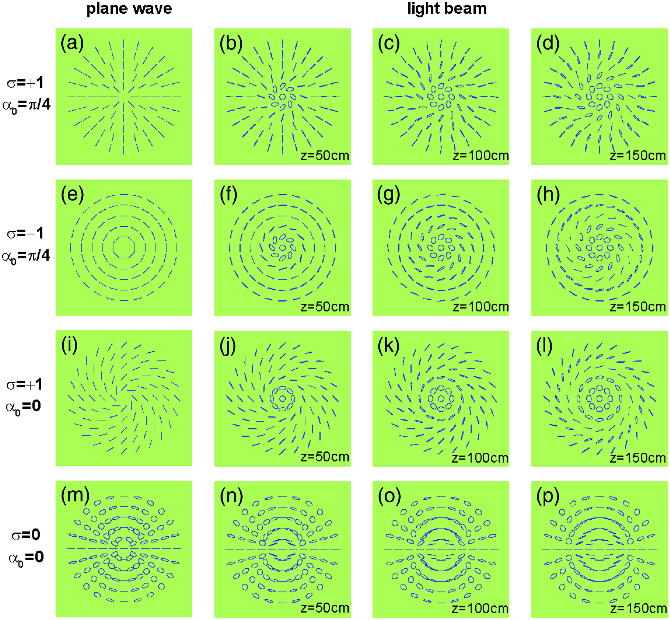
Figure 1.Polarization distributions of vector fields generated by $q$ -plates for different incident waves. The first column shows the theoretical results for an incident plane wave, while the others show an incident Gaussian beam. The four rows correspond to incidences of right, left, and right circular and linear polarizations $(σ = + 1, - 1, + 1, 0)$ , respectively. The $q$ -plates used have $q = 1$ and $α_{0} = π / 4$ in the upper two rows and $q = 1$ and $α_{0} = 0$ in the other rows. The dimension for all images is $w_{0} \times w_{0}$ , where $w_{0} = 1.75 mm$ .

The difference between the two results can be seen clearer in terms of the evolution of polarization on the Poincaré sphere. As an example, the polarization states along a radial line on the image plane in Figs. 1(i) and 1(j) are shown in Fig. 2(a). It shows that, for an incident plane wave, the exit polarization states along a radial line (for a given $θ$ ) correspond to a point on the Poincaré sphere; for an incident circularly polarized Gaussian beam, the polarization states along the same radial direction correspond to a curve starting from the north pole, after spiraling many rounds, ending at the south pole. One can show that the states for a different $θ$ follow a trajectory that is a rigid rotation of the above curve around the $S_{3}$ axis. Therefore, all the polarization states on a transverse plane cover the whole surface of the Poincaré sphere, so the resultant VB of Eq. (13) is a full Poincaré beam ^[43]. Note that for the full Poincaré beams in ^[43], the polarization states along radial lines map onto meridians on the Poincaré sphere, distinct from the spiraling curve in Fig. 2(a). Therefore, the present VB in Eq. (13) is a new family of full Poincaré beams.

Figure 2.Polarization evolution on the Poincaré sphere. (a) For the vector vortex beam in Fig. 1(j), the polarization states along a radial direction (from $r = 0$ to $\infty$ for a given $θ$ ) evolve from the north pole to the south pole. For the vector field in Fig. 1(i), the states in a radial direction correspond to a single point that does not change with propagation. (b) For the VB in Fig. 1(n), the polarization states on circles with different radii around the beam center evolve along different 8-shaped curves. Here, $r_{0} = 0.3 mm$ is the radius of the first circle in Fig. 1. For the vector field in Fig. 1(m), the states on all circles evolve along the same 8-shaped curve.

VBs with hybrid polarizations. If the incident light beam is linearly polarized ( $2 ϑ = π / 2$ , corresponding to the equator of the Poincaré sphere), Eq. (8) shows that the emerging light beam is hybridly polarized:

In comparison, the exit light for an incident plane wave can be obtained from Eq. (6) by setting $E_{0}$ constant:

Equivalently, $E_{p} (r, z) = E_{0} e^{- i π / 4} [\cos (α - ϕ + π / 4) e^{- i α} | + ⟩ + \sin (α - ϕ + π / 4) e^{i α} | - ⟩] = E_{0} e^{- i π / 4} R (- α) {[\cos (ϕ - α); i \sin (ϕ - α)]}^{T}$ . This indicates that the exit light has a transverse distribution of hybrid polarizations with azimuthal-variant orientations and ellipticities.

Generally, $A_{1} \neq A_{2}$ , so the polarization in Eq. (16) cannot be simplified as that in Eq. (17). They represent different hybrid polarizations. We present an example in the last row of Fig. 1. Figure 1(m) corresponds to the result of Eq. (17), while Figs. 1(n)–1(p) correspond to Eq. (16). Evidently, the two fields both vary azimuthally, but the polarizations in Figs. 1(n)–1(p) change with the radius $r$ and propagation distance $z$ , as well.

In order to visualize such a difference, we map the polarization states along circles with different radii in the beam cross section onto the Poincaré sphere in Fig. 2(b). It can been seen that the polarization around all circles for the incidence of a plane wave corresponds to an 8-shaped curve, which is mirror symmetric with respect to the $S_{1}$ axis, while the polarizations along different rings for an incident Gaussian beam correspond to entirely different 8-shaped curves. Interestingly, such curves degenerate into the equator for states on the beam periphery with a radius far larger than the beam waist.

3. EXPERIMENTAL RESULTS

To demonstrate the polarization distributions of VBs, we constructed $q$ -plates by using dielectric metasurfaces. These metasurfaces were fabricated by etching continuously varying grooves in a fused silica sample using a femtosecond laser ^[48]. The resulting self-assembled nanogratings produce a form birefringence with optical axes periodically varying in the azimuthal direction, as in Eq. (5). By controlling the etched depth of grooves, a retardation of $π / 2$ is achieved and then an effective inhomogeneous QWP is realized.

The experimental apparatus is depicted in Fig. 3. An He–Ne laser (632.8 nm, 17 mW, Thorlabs HNL210L-EC) outputs a linearly polarized fundamental Gaussian beam with a waist $w_{0} = 1.75 mm$ . A Glan laser polarizer (GLP1) and QWP1 are employed to obtain an appropriate incident polarization state. The laser beam then passes through the $q$ -plate, and the output intensity is recorded by a CCD camera (Coherent LaserCam HR). Another QWP (QWP2) and a polarizer (GLP2) are inserted to measure the Stokes parameters of the exit beam.

Figure 3.Schematic of experimental setup to generate VBs. The inset is a schematic drawing of the $q$ -plate with $q = 1$ and $α_{0} = π / 4$ . White short lines denote the orientations of local optical axes.

A. Vector Vortex Beams

First, we illuminated a $q$ -plate of $q = 1$ and $α_{0} = π / 4$ with left and right circularly polarized Gaussian beams to generate the vector polarization in Figs. 1(b) and 1(f). The transverse intensities of the resultant radial and azimuthal beams are measured at $z = 50 cm$ and shown in Fig. 4. It is seen that the intensities exhibit concentric rings determined by the hypergeometric function in Eq. (13). We also measured the Stokes parameters and then used them to retrieve the polarization states ^[38,39]. The results are depicted in Fig. 4. The experimental results agree with the theoretical ones very well.

Figure 4.Intensities and polarizations measured on the transverse plane $z = 50 cm$ . The top and bottom rows result from the incidence of right and left circularly polarized Gaussian beams, respectively. The left and right columns are the theoretical and experimental results, respectively. Here the $q$ -plate with $q = 1$ and $α_{0} = π / 4$ is used. The size for all images is $2.4 mm \times 2.3 mm$ .

To uncover its construction, we evaluated the VB by using a linear polarizer and the CCD. The result is shown in Fig. 5(d). An $S$ -shaped pattern typical for radial polarization is observed. This is due to the superposition of a vortex beam and a Gaussian beam with opposite circular polarizations ^[49], as indicated in Eq. (13). We also measured the two components, as presented in Figs. 5(e) and 5(f). The agreement between the experimental and theoretical results confirms the theory of Eq. (13).

Figure 5.For the radially polarized beam in Fig. 4(a), (a) is the intensity through a linear polarizer with the transmission axis indicated by the arrow; (b) and (c) are the intensities of the left and right circularly polarized components, respectively. The bottom row shows the experimental results corresponding to the top one.

Similar experiments were done for the azimuthally polarized beam in Fig. 4(d) and the results are presented in Fig. 6. Different from the radially polarized beam, the azimuthally polarized beam has a reversed $S$ -shaped pattern for the intensity through a linear polarizer; it has a left circularly polarized solid beam and a right circularly polarized vortex component.

Figure 6.For the azimuthally polarized beam Fig. 4(c), (a) is the intensity through a linear polarizer with the transmission axis indicated by the arrow; (b) and (c) are the intensities of the left and right circularly polarized components, respectively. In the bottom row are the experimental results corresponding to the top one.

To study the polarization evolution during propagation, we generated a spiral polarization determined by Eq. (15) for q = 1 and $α_{0} = 0$ and measured its transverse intensity at different propagation distances. The experimental results are given in Fig. 7. The overall tendencies of vector polarizations are in agreement with the theoretical ones. Nevertheless, there are some discrepancies, particularly in the case of $z = 150 cm$ . This may result from the fact that the intensity decays upon propagation, thus a small error in the measurement can lead to a very large deviation of the retrieved polarization state.

Figure 7.Transverse intensities and polarizations for a spirally polarized VB at different propagation distances. The top, middle, and bottom rows correspond to $z = 50$ , 100, and 150 cm, respectively. The left and right columns are the theoretical and experimental results, respectively. Here the incident Gaussian beam is right circularly polarized and the $q$ -plate with $q = 1$ and $α_{0} = 0$ is used. The size for all images is $2.4 mm \times 2.3 mm$ .

For the purpose of quantitative study, we drew the intensities in Fig. 7 along a radial line as a function of the radius. The results are shown in Figs. 8(a) and 8(b), where the experimental results agree remarkably well with the theoretical ones. Evidently, the intensity is not a single ring, but rather consists of concentric rings and a non-zero intensity center. According to Eqs. (8)–(12), the multi-ringed profile is mainly attributed to the term $- i E_{1 / 2} (r, z) / \sqrt{2}$ in Eq. (8). It can be understood as that the diffraction through the $q$ -plate not only converts the incident light into a vortex, but simultaneously imposes a modification of the confluent hypergeometric function in Eq. (12) onto the otherwise ideal single-ringed vortex ^[39,50]. As for the non-zero central intensity, it is the residual incident light $E_{i} (r, z) / \sqrt{2}$ in Eq. (8).

Figure 8.(a) Theoretical and (b) experimental results of the radial intensity distributions for the spirally polarized beam in Fig. 7. The intensities are normalized by the center intensity of the incident Gaussian beam. (c) Theoretical and (d) experimental results of the radial intensity distributions for the spirally polarized beam and its two circular polarization components measured at $z = 50 cm$ . On top are the local polarization states. (e) is the evolution of polarization states along a radial line ( $0 \leq r \leq 2.5 mm$ and $θ = π / 4$ ).

To shed light on the formation of the spiral polarization, we measured the transverse intensities of the circularly polarized components at $z = 50 cm$ , and the results are plotted in Fig. 8(d). The theoretical results calculated by Eq. (13) are shown in Fig. 8(c). According to the magnitudes of $| + ⟩$ and $| - ⟩$ , one can derive the polarization state along $r$ . For example, there is no $| - ⟩$ at point $A$ , so the polarization state is $| + ⟩$ ; there are equal magnitudes of $| + ⟩$ and $| - ⟩$ at point $B$ , so it is linear polarization. Similarly, one can conclude that it is right- and left-handed elliptical polarization from $A$ to $B$ and between $B$ and $D$ (including point $C$ , which has the maximum intensity), respectively. When approaching the periphery $E$ , the polarization state spirals near the equator, changing successively between right-handed and left-handed elliptical polarizations.

Then we mapped the polarization states onto the Poincaré sphere. As an example, we show in Fig. 8(e) the states along the radial line with the radial coordinate $r \leq 2.5 mm$ and the orientation $θ = π / 4$ . The intensity becomes very weak, even approaching zero, at the beam periphery. On the one hand, it may be out of our CCD’s capability of measurement. On the other hand, a weaker intensity is prone to bring a larger error in measurements. For these reasons, we chose the radial separation as $r \leq 2.5 mm$ . The variation tendency of the experimental polarization states in Fig. 8(e) shows reasonable agreement with the theoretical curve. Nevertheless, there are some deviations. These experimental errors may be ascribed to the measured intensity of the right circular polarization component, which is larger than that of the left one for $r > 1 mm$ , as evidenced in Fig. 8(d).

It is worth noting that the results of Figs. 8(a) and 8(c) not only apply to the beam in Fig. 7(a), but also to that in Fig. 4(a). This is because, in Eq. (13), the amplitudes of the components $| + ⟩$ and $| - ⟩$ for the incidence of $| + ⟩$ , $| A_{1} |$ , and $| A_{2} |$ are both independent of $α_{0}$ . Therefore, the intensities of the beam and the components of $| + ⟩$ and $| - ⟩$ in Fig. 7(a) are the same as those in Fig. 4(a). For the same reason, Figs. 8(a) and 8(c) can also represent the beam in Fig. 4(c), except exchanging $| + ⟩$ and $| - ⟩$ in Fig. 8(c). Hence, the handedness of the polarization ellipses in Fig. 4(c) is opposite to those in Figs. 7(a) and 4(a). Therefore, we conclude that the beams in Figs. 7(a), 4(a), and 4(c) have the same intensity and the same ellipticities of the polarization ellipses. However, the three beams do not have the same polarization distributions. This is because the phases of the $| + ⟩$ and $| - ⟩$ are different for these beams, whereby the polarization ellipses have different orientations, as indicated in Eq. (13).

B. VBs with Hybrid Polarizations

In the following we consider the incidence of a linearly polarized beam. The result for an incident horizontal polarization is shown in Fig. 9. Different from the above cylindrically symmetric VBs, the present beam is specularly symmetric. There are two off-center cores in its transverse intensity, like the overlap of two vortices reported in ^[51].

Figure 9.Transverse intensity and polarization distribution for the VB generated by a linearly polarized Gaussian beam passing through a $q$ -plate. (a) Theoretical results calculated by Eq. (16) and (b) experimental results measured at $z = 50 cm$ . Here, the $q$ -plate with $q = 1$ and $α_{0} = 0$ is used. The size for all images is $2.4 mm \times 2.3 mm$ .

To reveal the mechanism to this intensity distribution, we further measured the intensities of the circular polarization components. The results given in Fig. 10 show that the two components exhibit opposite $S$ -shaped profiles. According to Eqs. (8)–(10), the component $| + ⟩$ equals the superposition of a Gaussian beam and a vortex beam with a topological charge $l = - 2$ . Because the two beams, respectively, have planar and helical wavefronts, their interference results in a characteristic $S$ -shaped intensity pattern composed of two clockwise spiraling arms. This result is well known to the vortex beams. Actually, it consists of the common method to determine the topological charge of a vortex by the profile of the spiral arms ^[52]. For the component $| - ⟩$ , the constituent vortex beam has an opposite topological charge, so the resultant intensity exhibits an opposite $S$ -shaped pattern. If the two $S$ -shaped intensities were overlapped, one should obtain the total intensity with two minimum-intensity points in Fig. 9.

Figure 10.(a) and (b) are the transverse intensities for two circularly polarized components, respectively, and (c) the Stokes parameter $S_{3}$ , corresponding to the VB in Fig. 9. The second rows are correspondent experimental results.

The Stokes parameters were obtained by the standard experimental method to discover the polarization states. The polarizations retrieved are plotted on the intensity profile in Fig. 9. Obviously the VB consists of hybrid elliptical polarizations in the transverse plane, which is specularly symmetric as the intensity. In particular, the results of the Stokes parameter $S_{3}$ are given in Fig. 10. This shows that the two circularly components are separated completely. This is the well-known azimuthal spin splitting effect, namely, the azimuthal spin Hall effect of light ^[53,54]. Note that this effect was first investigated numerically in the Fraunhofer diffraction zone in ^[42]. Here we demonstrate this effect analytically and experimentally in the Fresnel diffraction zone.

To visualize the polarization evolution, we chose the third string of polarization states around the propagation axis for the VB in Fig. 9 and projected them onto the Poincaré sphere. The results are shown in Fig. 11. Despite some deviations, the experimental results agree well with the theoretical curve. Therefore, the theory of Eq. (16) or Eq. (8) is verified.

Figure 11.Polarization evolution on the Poincaré sphere. Shown are the theoretical and experimental results for the third string of polarization states (with a radius $r = 3 r_{0}$ ) on the beam cross section in Fig. 9.

4. CONCLUSION

We have investigated the polarization evolution of VBs generated with $q$ -plates. An explicit model of VBs beyond quarter-wave $q$ -plates was first established based on vector diffraction theory. Then it was found that VBs possess hybrid polarization distributions, which vary not only azimuthally but radially and axially, and are dependent on the value $q$ . Interestingly, for the incidence of circular polarizations, the exit vector vortex beam has polarization states that can cover the whole Poincaré sphere and then belong to full Poincaré beams. For the incidence of linear polarization, the VB is not cylindrically but is specularly symmetric and exhibits an azimuthal splitting of spin. By applying our model, the underlying mechanisms to the polarization and intensity profiles of VBs were revealed. Further experiments verified the theoretical results, where $q$ -plates were constructed by using dielectric metasurfaces.

The results are in sharp contrast with those for the incidence of a plane wave, where the vector field is only azimuthally varying. Our results demonstrate the importance of the practical spatial dimensions to VBs as well as full Poincaré beams. Since it reveals the underlying physics behind the VBs, the present model may be used to investigate the propagation dynamics of VBs. For example, it can be applied to dynamical effects of the aforementioned vector vortex beam since it has a radially variant polarization, which may produce orbital angular momentum ^[55,56]. Apart from the polarization, the results may also be applied to study the spin–orbital interactions involving $q$ -plates or metasurfaces ^[54], such as the spin-to-orbital angular momentum conversion ^[33,50] and the spin Hall effect of light ^[53,54].

References

[1] Q. Zhan. Cylindrical vector beams: from mathematical concepts to applications. Adv. Opt. Photon., 1, 1-57(2009).

[2] S. Quabis, R. Dorn, M. Eberler, O. Glöckl, G. Leuchs. Focusing light to a tighter spot. Opt. Commun., 179, 1-7(2000).

[3] R. Dorn, S. Quabis, G. Leuchs. Sharper focus for a radially polarized light beam. Phys. Rev. Lett., 91, 233901(2003).

[4] A. Bouhelier, M. Beversluis, A. Hartschuh, L. Novotny. Near-field second-harmonic generation induced by local field enhancement. Phys. Rev. Lett., 90, 013903(2003).

[5] L. Novotny, M. R. Beversluis, K. S. Youngworth, T. G. Brown. Longitudinal field modes probed by single molecules. Phys. Rev. Lett., 86, 5251-5254(2001).

[6] K. S. Youngworth, T. G. Brown. Focusing of high numerical aperture cylindrical vector beams. Opt. Express, 7, 77-87(2000).

[7] Q. Zhan. Trapping metallic Rayleigh particles with radial polarization. Opt. Express, 12, 3377-3382(2004).

[8] C. Hnatovsky, V. G. Shvedov, W. Krolikowski, A. Rode. Revealing local field structure of focused ultrashort pulses. Phys. Rev. Lett., 106, 123901(2011).

[9] V. D’Ambrosio, N. Spagnolo, L. D. Re, S. Slussarenko, Y. Li, L. C. Kwek, L. Marrucci, S. P. Walborn, L. Aolita, F. Sciarrino. Photonic polarization gears for ultra-sensitive angular measurements. Nat. Commun., 4, 2432(2013).

[10] D. P. Biss, K. S. Youngworth, T. G. Brown. Dark-field imaging with cylindrical-vector beams. Appl. Opt., 45, 470-479(2006).

[11] X. Li, Y. Cao, M. Gu. Superresolution-focal-volume induced 3.0 Tbytes/disk capacity by focusing a radially polarized beam. Opt. Lett., 36, 2510-2512(2011).

[12] X. Li, T. H. Lan, C. H. Tien, M. Gu. Three-dimensional orientation-unlimited polarization encryption by a single optically configured vectorial beam. Nat. Commun., 3, 998(2012).

[13] G. Milione, T. A. Nguyen, J. Leach, D. A. Nolan, R. R. Alfano. Using the nonseparability of vector beams to encode information for optical communication. Opt. Lett., 40, 4887-4890(2015).

[14] J. T. Barreiro, T. C. Wei, P. G. Kwiat. Remote preparation of single-photon “hybrid” entangled and vector-polarization states. Phys. Rev. Lett., 105, 030407(2010).

[15] V. D’Ambrosio, E. Nagali, S. P. Walborn, L. Aolita, S. Slussarenko, L. Marrucci, F. Sciarrino. Complete experimental toolbox for alignment-free quantum communication. Nat. Commun., 3, 961(2012).

[16] R. Oron, S. Blit, N. Davidson, A. A. Friesem, Z. Bomzon, E. Hasman. The formation of laser beams with pure azimuthal and radial polarization. Appl. Phys. Lett., 77, 3322-3324(2000).

[17] Y. Kozawa, S. Sato. Generation of a radially polarized laser beam by use of a conical Brewster prism. Opt. Lett., 30, 3063-3065(2005).

[18] T. Grosjean, D. Courjon, M. Spajer. An all-fiber device for generating radially and other polarized light beams. Opt. Commun., 203, 1-5(2002).

[19] S. Ramachandran, P. Kristensen, M. F. Yan. Generation and propagation of radially polarized beams in optical fibers. Opt. Lett., 34, 2525-2527(2009).

[20] S. C. Tidwell, D. H. Ford, W. D. Kimura. Generating radially polarized beams interferometrically. Appl. Opt., 29, 2234-2239(1990).

[21] C. Maurer, A. Jesacher, S. Fürhapter, S. Bernet, M. Ritsch-Marte. Tailoring of arbitrary optical vector beams. New J. Phys., 9, 78(2007).

[22] X. L. Wang, J. Ding, W. J. Ni, C. S. Guo, H. T. Wang. Generation of arbitrary vector beams with a spatial light modulator and a common path interferometric arrangement. Opt. Lett., 32, 3549-3551(2007).

[23] G. Milione, S. Evans, D. A. Nolan, R. R. Alfano. Higher order Pancharatnam-Berry phase and the angular momentum of light. Phys. Rev. Lett., 108, 190401(2012).

[24] D. Maluenda, I. Juvells, R. Martínez-Herrero, A. Carnicer. Reconfigurable beams with arbitrary polarization and shape distributions at a given plane. Opt. Express, 21, 5424-5431(2013).

[25] I. Moreno, J. A. Davis, D. M. Cottrell, R. Donoso. Encoding high-order cylindrically polarized light beams. Appl. Opt., 53, 5493-5501(2014).

[26] Z. Chen, T. Zeng, B. Qian, J. Ding. Complete shaping of optical vector beams. Opt. Express, 23, 17701-17710(2015).

[27] P. Li, Y. Zhang, S. Liu, C. Ma, L. Han, H. Cheng, J. Zhao. Generation of perfect vectorial vortex beams. Opt. Lett., 41, 2205-2208(2016).

[28] G. Machavariani, Y. Lumer, I. Moshe, A. Meir, S. Jackel. Efficient extracavity generation of radially and azimuthally polarized beams. Opt. Lett., 32, 1468-1470(2007).

[29] J. A. Davis, N. Hashimoto, M. Kurihara, E. Hurtado, M. Pierce, M. M. Sánchez-López, K. Badham, I. Moreno. Analysis of a segmented q-plate tunable retarder for the generation of first-order vector beams. Appl. Opt., 54, 9583-9590(2015).

[30] Z. Bomzon, G. Biener, V. Kleiner, E. Hasman. Radially and azimuthally polarized beams generated by space-variant dielectric subwavelength gratings. Opt. Lett., 27, 285-287(2002).

[31] E. Hasman, G. Biener, A. Niv, V. Kleiner. Space-variant polarization manipulation. Prog. Opt., 47, 215-289(2005).

[32] A. Niv, G. Biener, V. Kleiner, E. Hasman. Manipulation of the Pancharatnam phase in vectorial vortices. Opt. Express, 14, 4208-4220(2006).

[33] L. Marrucci, C. Manzo, D. Paparo. Optical spin-to-orbital angular momentum conversion in inhomogeneous anisotropic media. Phys. Rev. Lett., 96, 163905(2006).

[34] M. Stalder, M. Schadt. Linearly polarized light with axial symmetry generated by liquid-crystal polarization converters. Opt. Lett., 21, 1948-1950(1996).

[35] F. Cardano, E. Karimi, S. Slussarenko, L. Marrucci, C. de Lisio, E. Santamato. Polarization pattern of vector vortex beams generated by q-plates with different topological charges. Appl. Opt., 51, C1-C6(2012).

[36] V. D’Ambrosio, F. Baccari, S. Slussarenko, L. Marrucci, F. Sciarrino. Arbitrary, direct and deterministic manipulation of vector beams via electrically-tuned q-plates. Sci. Rep., 5, 7840(2015).

[37] D. Naidoo, F. S. Roux, A. Dudley, I. Litvin, B. Piccirillo, L. Marrucci, A. Forbes. Controlled generation of higher-order Poincaré sphere beams from a laser. Nat. Photonics, 10, 327-332(2016).

[38] Y. Liu, X. Ling, X. Yi, X. Zhou, H. Luo, S. Wen. Realization of polarization evolution on higher-order Poincaré sphere with metasurface. Appl. Phys. Lett., 104, 191110(2014).

[39] W. Shu, Y. Liu, Y. Ke, X. Ling, Z. Liu, B. Huang, H. Luo, X. Yin. Propagation model for vector beams generated by metasurfaces. Opt. Express, 24, 21177-21189(2016).

[40] G. Li, M. Kang, S. Chen, S. Zhang, E. Y. B. Pun, K. W. Cheah, J. Li. Spin-enabled plasmonic metasurfaces for manipulating orbital angular momentum of light. Nano Lett., 13, 4148-4151(2013).

[41] M. Kang, J. Chen, B. Gu, Y. Li, L. T. Vuong, H. T. Wang. Spatial splitting of spin states in subwavelength metallic microstructures via partial conversion of spin-to-orbital angular momentum. Phys. Rev. A, 85, 035801(2012).

[42] X. Ling, X. Zhou, H. Luo, S. Wen. Steering far-field spin-dependent splitting of light by inhomogeneous anisotropic media. Phys. Rev. A, 86, 053824(2012).

[43] A. M. Beckley, T. G. Brown, M. A. Alonso. Full Poincaré beams. Opt. Express, 18, 10777-10785(2010).

[44] E. J. Galvez, S. Khadka, W. H. Schubert, S. Nomoto. Poincaré-beam patterns produced by nonseparable superpositions of Laguerre-Gauss and polarization modes of light. Appl. Opt., 51, 2925-2934(2012).

[45] W. Shu, Y. Ke, Y. Liu, X. Ling, H. Luo, X. Yin. Radial spin Hall effect of light. Phys. Rev. A, 93, 013839(2016).

[46] J. W. Goodman. Introduction to Fourier Optics(2005).

[47] I. S. Gradshteyn, I. M. Ryzhik. Table of Integrals, Series, and Products(2007).

[48] M. Beresna, M. Gecevičius, P. G. Kazansky. Polarization sensitive elements fabricated by femtosecond laser nanostructuring of glass. Opt. Mater. Express, 1, 783-795(2011).

[49] M. Beresna, M. Gecevičius, P. G. Kazansky, T. Gertus. Radially polarized optical vortex converter created by femtosecond laser nanostructuring of glass. Appl. Phys. Lett., 98, 201101(2011).

[50] E. Karimi, B. Piccirillo, L. Marrucci, E. Santamato. Light propagation in a birefringent plate with topological charge. Opt. Lett., 34, 1225-1227(2009).

[51] D. Rozas, C. T. Law, G. A. Swartzlander. Propagation dynamics of optical vortices. J. Opt. Soc. Am. B, 14, 3054-3065(1997).

[52] M. Padgett, J. Courtial, L. Allen. Light’s orbital angular momentum. Phys. Today, 57, 35-40(2004).

[53] X. Ling, X. Zhou, W. Shu, H. Luo, S. Wen. Realization of tunable photonic spin Hall effect by tailoring the Pancharatnam-Berry phase. Sci. Rep., 4, 5557(2014).

[54] K. Y. Bliokh, F. J. Rodríguez-Fortuño, F. Nori, A. V. Zayats. Spin-orbit interactions of light. Nat. Photonics, 9, 796-808(2015).

[55] X. L. Wang, J. Chen, Y. Li, J. Ding, C. S. Guo, H. T. Wang. Optical orbital angular momentum from the curl of polarization. Phys. Rev. Lett., 105, 253602(2010).

[56] B. Gu, B. Wen, G. Rui, Y. Xue, Q. Zhan, Y. Cui. Varying polarization and spin angular momentum flux of radially polarized beams by anisotropic Kerr media. Opt. Lett., 41, 1566-1569(2016).