In three-dimensional (3D) measurement, fringe projection profilometry (FPP) has been widely used in industrial detection, quality control, machine vision, 3D printing, film and television special effects, biomedical industry and other fields because of its rapidity, non-contact, and high accuracy^[1-4]. At present, Fourier transform profilometry (FTP)^[5-6] and phase measurement profilometry (PMP)^[7-8] are widely used in FPP. PMP is a method to measure the 3D information of the object using a phase-shifting method and has the advantages of a large field of view and high-measurement accuracy, which is the research focus in the field of 3D measurement. The system then must be calibrated to obtain the relationship between the absolute phase and the true height of the measured object. Therefore, system calibration plays a very important role in the measurement process. The existing calibration of methods can be roughly divided into two types: the calibration technology based on stereo vision(SV) and the calibration of phase-to-height mapping (PHM).

PHM or system parameter calibration directly establishes the phase-height mapping relationship through a mathematical model, so there is no need to calibrate the projector. Based on the conventional formula^{[5, 9-10]} of PHM, Zhou^[11] proposed a linear phase-height mapping relationship based on an ideal geometric optical imaging system, and proposed a direct phase-height algorithm. Asundi^[12] proposed a unified calibration technology based on ray tracing triangle profilometry, which can measure quickly and accurately without determining geometric parameters. Li^[13] adopted a conic-fitting method to propose a new bidirectional nonlinear phase-height mapping algorithm and an accurate lateral coordinate calibration method to obtain the 3D coordinates of the measured object. But these methods have not eliminated the influence of system geometry. Du^[14] proposed a two-step calibration procedure for 3D surface profilometry and used the phase difference to convert between the world coordinate system and the image coordinate system to obtain accurate 3D point cloud data. Gai^[15] built a novel geometrical model in 3D space to determine the mapping and greatly reduced the constraints of traditional models. Zhang^[16] used a checkerboard calibration target and a white plane with discrete hollow ring markers to construct a single polynomial function between the phase difference and the depth of the measured object. Léandry^[17] performed a systematic study of different degrees (1,2,3,4) of a polynomial form. Although the best results were obtained with the polynomial degree 4, Léandry selected the degree 3 because its result was simpler. Siegmann^[18] considered that the fringe pattern period of the reference plane would change when the fringe pattern was tilted and projected, and proposed a 2D image correction method for data image correction. Gonzalez^[19] proposed a method that can eliminate the effect of projector lens distortion without projector calibration. Point cloud registration is a key step in 3D reconstruction. It is currently one of the main methods of point cloud registration to register point cloud from multiple angles to a reference coordinate system using a turntable. Because the system calibration will affect the depth information accuracy of a single angle, thereby affecting the registration accuracy. Current calibration techniques rely on back-projection SV methods and PHM. SV calibration method is more flexible in that the calibration target can be arbitrarily positioned. However, it generally does not achieve the same accuracy level as PHM. Although PHM method produces highly accurate measurement within the calibration volume, it is cumbersome to implement as they require precise moving stage and calibration plane. We propose a calibration method based on turntable. Then, in the measurement system using turntable to complete the point cloud registration, the system calibration can be completed without additional moving stage. The method has the flexibility and saves the cost of equipment.

Section 1 introduces the principle of PMP method. We describe the principles of the proposed method and traditional method in section 2. Section 3 gives the accuracy evaluation by experiments, and verifies the practicability of the proposed method. Section 4 contains the conclusion of this paper.

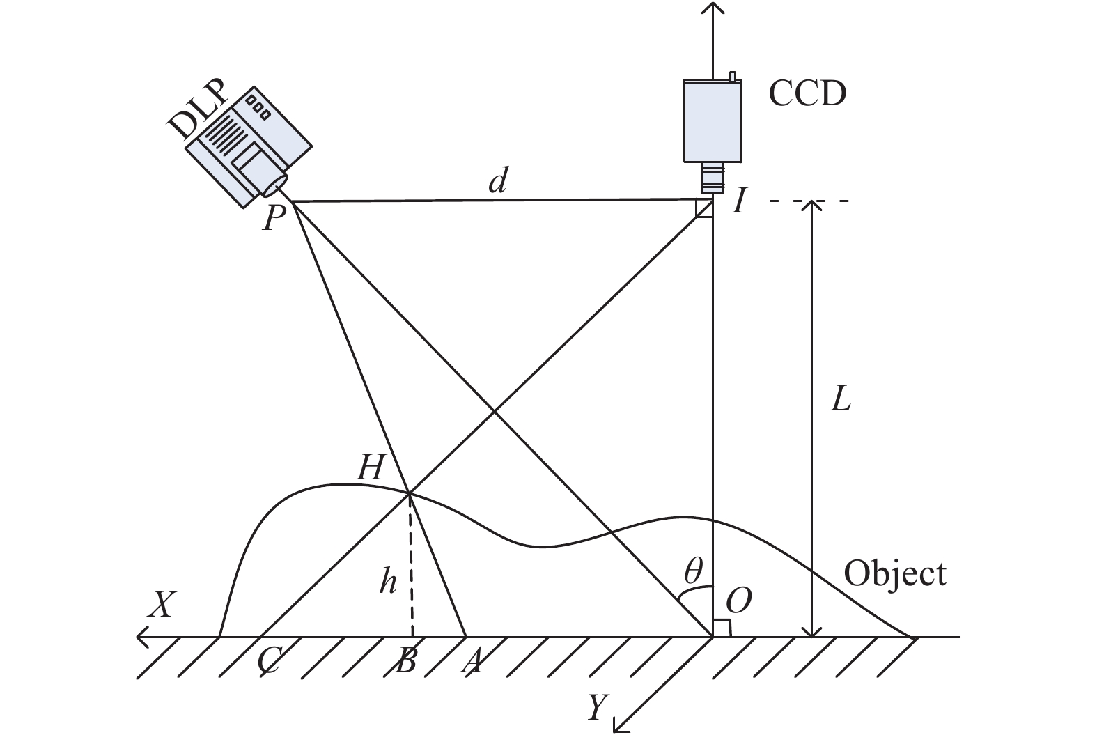
The light path principle of PMP is shown in Fig.1. A random point $ H $ on the object surface, and the distance from the point to the reference plane is h. According to the triangle principle^[5], the phase-height formula is shown as follows:

$ h(u,v) = \frac{{L(u,v)\Delta \varphi (u,v)}}{{2\pi fd(u,v) + \Delta \varphi (u,v)}} $ (1)

Where, $ L(u,v) $ and $ d(u,v) $ are the system parameters and can be obtained by calibration, $ f $ is the frequency of fringe pattern and $ (u,v) $ denotes the pixel coordinates of a point in the distorted fringe pattern. Eq. (1) shows that in order to obtain the true height information $ h $ of the measured object, the phase difference $\Delta \varphi (u,v)$ of the measured object must first be obtained.

By using the projection system of Fig. 1, the sinusoidal fringes with phase shift are projected on the point H of the measured object surface. The encoded sinusoidal fringes are modulated by the measured object surface, and the light intensity can be calculated as follows:

$ I(u,v) = a(u,v) + b(u,v)\cos (\varphi (u,v) + \delta ) $ (2)

Where, $ a(u,v) $ represents the background light intensity at any point A on the reference plane, and for a particular point, the background light intensity is constant, $ b(u,v) $ is the intensity amplitude of the projector, $ \varphi (u,v) $ is the phase distribution modulated by the measured object, $ \delta $ is the phase shift. As for the $ N(N \geqslant 3) $-step phase-shifting method, the light intensity is presented as follows:

$ \begin{split} {I_n}(x,y) =& a(x,y) + b(x,y)\cos \Bigg[\varphi (x,y) +\\ & \dfrac{{2\pi (n - 1)}}{N}\Bigg](n = 1,2,3 \cdots N) \end{split} $ (3)

In this paper, a four $ (N = 4) $-step phase method is used, so the phase difference between two adjacent fringe pattern images is $ {\pi / {\text{2}}} $, and the corresponding light intensity can be described as follows:

$ \left\{ {\begin{array}{*{20}{c}} {{I_1} = a(x,y) + b(x,y)\cos [\varphi (x,y) + {\text{0}}]} \\ {{I_2} = a(x,y) + b(x,y)\cos \left[\varphi (x,y) + \dfrac{\pi }{2}\right]} \\ {{I_3} = a(x,y) + b(x,y)\cos [\varphi (x,y) + \pi ]} \\ {{I_4} = a(x,y) + b(x,y)\cos \left[\varphi (x,y) + \dfrac{{3\pi }}{2}\right]} \end{array}} \right. $ (4)

Solving the presented equations uniquely obtains the expression for the phase map $ \phi (u,v) $ as follows:

$ \phi (x,y) = \arctan \left[ {\frac{{{I_4}(x,y) - {I_2}(x,y)}}{{{I_1}(x,y) - {I_3}(x,y)}}} \right] $ (5)

This process is called "phase unwrapping" because the computed phase value has the range $ \left( { - \pi ,\pi } \right] $ and needs to be calculated to obtain the continuous phase value $ \varphi (u,v) $ as follows:

$ \varphi (x,y) = \phi (x,y) + k(x,y) \cdot 2\pi $ (6)

A continuous phase map can be obtained by adopting the three frequency heterodyne phase unwrapping method^[20], and the phase-height mapping could convert the absolute phase to the depth information.

In the measurement system shown in Fig. 1, Eq. (1) is still widely used, and its deformation formula is as follows:

$ \frac{1}{{h(u,v)}} = \frac{1}{{L(u,v)}} + \frac{{2\pi fd(u,v)}}{{L(u,v)}} \cdot \frac{1}{{\varDelta \varphi (u,v)}} $ (7)

Letting ${C_1}(u,v) = {{\text{1}} / {L(u,v)}}$ and ${C_{\text{2}}}(u,v) = {{2\pi f \cdot}} $$ {{ d(u,v)} /} { {L(u,v)}}$, Eq. (7) can be simplified as follows:

$ \frac{1}{{h(u,v)}} = {C_1}(u,v) + {C_2}(u,v) \cdot \frac{1}{{\Delta \varphi (u,v)}} $ (8)

Where, $ {C_1}(u,v) $ and $ {C_{\text{2}}}(u,v) $ can be obtained by the system calibration method. In the case, a calibration method is proposed by determining the distributions of the parameters $ {C_1}(u,v) $ and $ {C_{\text{2}}}(u,v) $. Its principle is illustrated in Fig. 2, and the procedure can be summarized as follows. First, a standard plane is positioned at $ h = 0 $, and then the distributions of reference phase can be measured and denoted as $ {\varphi _0}(u,v) $. Second, by shifting the plane to different positions with given depths $ {h_i} $, the phase distributions can be obtained and denoted as $ {\varphi _i}(u,v) $, where $ i = 1,2, \cdots ,n $. Accordingly, the phase differences are given by

$ \Delta {\varphi _i}(u,v) = {\varphi _i}(u,v) - {\varphi _0}(u,v)\begin{array}{*{20}{c}} {}&{i = 1,...,n} \end{array} $ (9)

Third, because there are two parameters to be determined, the parameters can be estimated from the measurement result when the condition $ n \geqslant 2 $ is satisfied.

By using the geometric dimension relationship of the electric turntable, the measured surface of the calibration plate passes through the axis of the turntable. A customized calibration plate is placed vertically on the high-precision electric turntable. The process of the new calibration method is shown in Fig. 3.

The principle of the new phase-height mapping calibration method is as follows:

Step 1: First, the phase shift method is used to measure the surface of the calibration plane, and the phase information of the measured surface at this time is collected and recorded as $ {\varphi _{\text{0}}}(u,v) $.

Step 2: The electric turntable drives the calibration plate to rotate at a certain angle, as shown in Fig. 3. We collect the phase information of the calibration plate’s measured plane at this moment and record it as $ \varphi (u,v) $.

Step 3: As shown in Fig. 4, Figs. 4(a) and 4(b) are the circle centers of calibration plate image and its partial enlargement, respectively.

The camera is used to capture the marker points in the image, and the pixel coordinates of the center of each marker point are identified and saved. After obtaining the pixel coordinates of the marker point, the phase value $ {\varphi _i}(u,v) $ at the marker point on the calibration plate after rotation is known via $ \varphi (u,v) $.

Step 4: As shown in Fig. 5, the height $ {h_i}(x,y) $ from the marker point $ {q_i}(i = 1,2, \cdots ,n) $ to the reference plane is following:

$ {h_i} = a\sin \theta + (i - 1)l\sin \theta (i = 1,2, \cdots ,n) $ (10)

Where, $ \theta $ is the rotation angle of the calibration plate, $ \theta $ is determined by the precision turntable, and $ a $ is the distance from the center of the first marker point to the axis of the turntable. The distance between the centers of the marker point is equal, and its value is $ l $, and $ n $ is the number of marker points.

Step 5: The phase difference $\Delta {\varphi _i}(u,v)$ can be obtained by subtracting the phase value $ {\varphi _0}(u,v) $ of the corresponding point on the reference plane from the phase value $ {\varphi _i}(u,v) $ of the marker point $ {q_i}(i = 1,2, \cdots ,n) $,whose height is $ {h_i}(u,v) $ through the $ i $ marker point. Therefore, Eq. (8) can be rewritten as follows:

$ \frac{1}{{{h_i}(u,v)}} = {C_1}(u,v) + {C_2}(u,v) \cdot \frac{1}{{\Delta {\varphi _i}(u,v)}} $ (11)

As shown in Fig. 1, because the parameters $ {C_1}(u,v) $ and $ {C_{\text{2}}}(u,v) $ are parameters related to the two constants $ L(u,v) $ and $ d(u,v) $, so they are also constants in theory. To calculate the measured object absolute height out-of-reference plane with Eq. (8), the parameters $ {C_1}(u,v) $ and $ {C_{\text{2}}}(u,v) $ must be determined first. However, physically measuring those parameters, such as the parameter $ d $, should be avoided in order to ensure high measurement accuracy and practicability. To cope with this issue, the parameters $ {C_1}(u,v) $ and $ {C_{\text{2}}}(u,v) $ will be determined through using a least-squares inverse approach based on $ n(n \geqslant 2) $ marker points whose heights are precisely known. The least-squares method is employed here because it utilizes many marker points to enhance the detection accuracy of the parameters $ {C_1}(u,v) $ and $ {C_{\text{2}}}(u,v) $. The least-squares error can be expressed as follows:

$ S = \sum\limits_{i = 1}^n {\left[ {\frac{1}{{L(u,v)}} + \frac{{2\pi fd(u,v)}}{{L(u,v)}} \cdot \frac{1}{{\Delta \varphi (u,v)}} - \frac{1}{{{h_i}(u,v)}}} \right]} $ (12)

Where $ {h_i}(u,v) $ denotes the absolute height out-of-reference-plane of the marker points, $ i $ is the ordinal number of each marker point, $ n $ is the total number of the marker points used in the calculation, and a larger $ n $ generally yields a higher accuracy. The parameters $ {C_1}(u,v) $ and $ {C_{\text{2}}}(u,v) $ in the equation can be determined by using a nonlinear least-squares algorithm such as the Levenberg–Marquardt method.

To verify the correctness of the proposed method, physical measurements were carried out. As shown in Fig.1, a measurement system based on turntable is established, the measurement system consists of computer, camera, projector and turntable. The projector model is DLP lightcraft 4500 with a resolution of 912×1140 pixel. The camera is an industrial CMOS camera (MER-131-210U3M) with a resolution of 1280×1024 pixel. The model of turntable is RAP125 (repeated positioning accuracy is less than 0.003°), and the control box is SC300. The measured object includes a block and a sphere, the purpose of measuring the calibration plate is to evaluate the measurement accuracy of the proposed method.

First, a four-step phase-shifting fringe patterns are projected onto a calibration plane, also referred to as the reference plane, and a fringe pattern is captured with a camera. Then, the calibration plane is moved 15 mm, 20 mm, 25 mm, 30 mm and 35 mm in turn, and the four-step phase-shifting fringe patterns are projected onto the calibration plane corresponding to the moving position. Finally, the phase values of the 6 calibration planes including the reference plane are obtained, and the phase values of the 5 calibration planes are subtracted from the phase values of the reference plane to obtain the continuous phase differences of the other 5 calibration planes relative to the reference plane. The continuous phase differences of the 5 calibration planes and the heights of the corresponding calibration planes are substituted into Eq. (8), and the traditional phase-height mapping relationship can be established by calculating parameters $ {C_1}(u,v) $ and $ {C_{\text{2}}}(u,v) $ with the least-squares method.

The measurement results obtained by the traditional phase-height calibration method are shown in Fig. 6. Figure 6(a) shows a deformed fringe pattern modulated by the block with a height of 10 mm. Figure 6(b) is part of a deformed fringe pattern. Figure 6(c) shows the continuous phase value of a block obtained by PMP. Figure 6(d) is the 3D point cloud data of a block.

The measurement results obtained by using the proposed phase-height calibration method are shown in Fig. 7. Figure 7(a) shows the new calibration system, and the distance from the center of the first marker point on the left to the axis of the turntable is 20 mm, the actual distance between the centers of the marker points is 10 mm, and the rotating angle θ of the turntable is 30°. Figure 7(b) shows the 3D point cloud data of the block with a height of 10 mm.

In 3D measurement, the root mean square error (RMSE) is commonly used to assess the measurement accuracy

$ \sigma = \sqrt {\sum {{{\left[ {h(u,v) - A} \right]}^2}/m} } $ (15)

Where h(u,v) is the reconstruction height of the block, A is the height of the white block with a value is of 10 mm, and m is the total number of pixels in the plane. Substituting the measurement results into Eq. (15) shows that the 3D reconstruction of the block with a height of 10 mm using the traditional method has an average height of 10.018 mm, and a RMSE of 0.043 mm. Similarly, the measurement results of the proposed method show an average height of 10.047 mm, and a standard deviation of 0.072 mm.

The traditional phase-height mapping calibration method and the new phase-height mapping calibration method are respectively used to reconstruct the calibration plane with a height of 10 mm. The comparison results are shown in Tab. 1.

Table 1 shows that no matter whether the traditional method or the proposed method is used, the 3D information of the measured object can be effectively obtained, and the measurement accuracy can be guaranteed. However, the table shows that the traditional calibration method is superior to the proposed calibration method in terms of average value, or RMSE, while the proposed method is more convenient and saves more time.

To verify the utility of the method, the measurement data of the sphere shown in Fig. 8, Figure 8(a) shows part of a sphere, whose diameter is 60.027 mm. Figure 8(b) shows a frame deformed fringe of the sphere, and Fig. 8(c) shows a phase distribution of the sphere. Figure 9 shows the 3D reconstruction results of the sphere, Figure 9(a) shows 3D shape by the traditional method. And Fig. 9(b) shows 3D shape by the proposed method, Figure 9 shows that both methods are good at restoring the 3D shape of the object.

To compare the difference between the two methods more clearly, the cutaway view of a column in the green circle of Fig. 9 was extracted from the 3D shape recovered by the two methods, and the comparison result is shown in Fig. 10. The measurement results show that the maximum height of the sphere surface is 60.071 mm obtained by the traditional method and 60.095 mm obtained by the proposed method, respectively. For the traditional method, due to need to move the standard plane several times (starting from the h₀ position), the measurement data fluctuates greatly due to the influence of dither and mechanical error. The new method only needs to rotate an angle $ \theta $ accurately, which is easy to realize with a precision turntable. The subsequent calculation processes are obtained by fitting and optimization algorithm, so the measurement data is relatively smoother.

In addition, another evaluation experiment is carried out by measuring a sculpture using the proposed method, as illustrated in Fig. 11. Figure 11(a) and 11(b) are the captured deformed pattern and the reconstructed 3D shape, respectively. Obviously, the proposed method can obtain satisfactory 3D shape of the measured object.

The traditional phase-height mapping calibration method generally uses a moving stage to drive the calibration plate to move several times within the depth of field of the camera, but this method has problems of complicated operation and inconvenient carrying. The proposed calibration method only needs to use a turntable to rotate the calibration plane once, the camera only needs to capture two sets of images, greatly improving the calibration speed of the system, but the measurement accuracy of the proposed calibration method is less than the traditional method.

Comparing these two methods, each has several unique advantages. In some fields, to achieve the registration of 3D point cloud, a structured light system based on a turntable is widely applied. In contrast to traditional method, the proposed method can achieve system calibration without the moving stage, and the error is also within tolerance.

On behalf of all authors, the corresponding author states that there is no conflict of interest.

References

[1] F Chen, G M Brown, M Song. Overview of 3-D shape measurement using optical methods. Optical Engineering, 39, 10-22(2000).
[2] Yongkai Yin, Zonghua Zhang, Xiaoli Liu, et al. Review of the system model and calibration for fringe projection profilometry. Infrared and Laser Engineering, 49, 0303008(2020).
[3] D Hong, H Lee, M Y Kim, et al. Sensor fusion of phase measuring profilometry and stereo vision for three-dimensional inspection of electronic components assembled on printed circuit boards. Applied Optics, 48, 4158-4169(2009).
[4] Chao Zuo, Xiaolei Zhang, Yan Hu, et al. Has 3D finally come of age?——An introduction to 3D structured-light sensor. Infrared and Laser Engineering, 49, 0303001(2020).
[5] M Takeda, K Mutoh. Fourier transform profilometry for the automatic measurement of 3-D object shapes. Applied Optics, 22, 3977-3982(1983).
[6] S Cao, Y Cao, Q Zhang. Fourier transform profilometry of a single-field fringe for dynamic objects using an interlaced scanning camera. Optics Communications, 367, 130-136(2016).
[7] V Srinivasan, H C Liu, M Halioua. Automated phase-measuring profilometry of 3-D diffuse objects. Applied Optics, 23, 3105-3108(1984).
[8] H Zhou, J Gao, H Hu, et al. Fast phase-measuring profilometry through composite color-coding method. Optics Communications, 440, 220-228(2019).
[9] G Sansoni, L Biancardi, U Minoni, et al. A novel, adaptive system for 3-D optical profilometry using a liquid crystal light projector. IEEE Transactions on Instrumentation and Measurement, 43, 558-566(1994).
[10] H Liu, W Su, K Reichard, et al. Calibration-based phase-shifting projected fringe profilometry for accurate absolute 3D surface profile measurement. Optics Communications, 216, 65-80(2003).
[11] W Zhou, X Su. A direct mapping algorithm for phase-measuring profilometry. Journal of Modern Optics, 41, 89-94(1994).
[12] A Asundi, Z Wensen. Unified calibration technique and its applications in optical triangular profilometry. Applied Optics, 38, 3556-3561(1999).
[13] W Li, X Su, Z Liu. Large-scale three-dimensional object measurement: A practical coordinate mapping and image data-patching method. Applied Optics, 40, 3326-3333(2001).
[14] H Du, Z Wang. Three-dimensional shape measurement with an arbitrarily arranged fringe projection profilometry system. Optics Letters, 32, 2438-2440(2007).
[15] Gai S, Da F. Threedimensional surface measurement system based on projected fringe model[C]3rd International Symposium on Advanced Optical Manufacturing Testing Technologies: Optical Test Measurement Technology Equipment, 2007, 6723: 67231X.
[16] Z Zhang, S Huang, S Meng, et al. A simple, flexible and automatic 3D calibration method for a phase calculation-based fringe projection imaging system. Optics Express, 21, 12218-12227(2013).
[17] I Léandry, C Brèque, V Valle. Calibration of a structured-light projection system: development to large dimension objects. Optics and Lasers in Engineering, 50, 373-379(2012).
[18] P Siegmann, L Felipe-Sese, F Diaz-Garrido. Improved 3D displacement measurements method and calibration of a combined fringe projection and 2D-DIC system. Optics and Lasers in Engineering, 88, 255-264(2017).
[19] A Gonzalez, J Meneses. Accurate calibration method for a fringe projection system by projecting an adaptive fringe pattern. Applied Optics, 58, 4610-4615(2019).
[20] J M Huntley, H O Saldner. Temporal phase-unwrapping algorithm for automated interferogram analysis. Applied Optics, 32, 3047-3052(1993).
Set citation alerts for the article
Please enter your email address
© Copyright 2018-2021 | Chinese Laser Press. All Rights Reserved 沪ICP备15018463号-20