• Advanced Photonics
  • Vol. 2, Issue 2, 024002 (2020)
Kang Lin1、†, Ilia Tutunnikov2, Junyang Ma1、3, Junjie Qiang1, Lianrong Zhou1, Olivier Faucher3、*, Yehiam Prior1、2、*, Ilya Sh. Averbukh2、*, and Jian Wu1、4、*
Author Affiliations
  • 1East China Normal University, State Key Laboratory of Precision Spectroscopy, Shanghai, China
  • 2Weizmann Institute of Science, Department of Chemical and Biological Physics, Rehovot, Israel
  • 3Université de Bourgogne Franche-Comté, Laboratoire Interdisciplinaire CARNOT de Bourgogne, UMR 6303 CNRS, Dijon, France
  • 4Shanxi University, Collaborative Innovation Center of Extreme Optics, Taiyuan, Shanxi, China
  • show less
    DOI: 10.1117/1.AP.2.2.024002 Cite this Article Set citation alerts
    Kang Lin, Ilia Tutunnikov, Junyang Ma, Junjie Qiang, Lianrong Zhou, Olivier Faucher, Yehiam Prior, Ilya Sh. Averbukh, Jian Wu. Spatiotemporal rotational dynamics of laser-driven molecules[J]. Advanced Photonics, 2020, 2(2): 024002 Copy Citation Text show less
    Approaches for inducing molecular UDR. (a) Double-pulse scheme for excitation of unidirectional molecular rotation (adapted from Ref. 53, CC BY). (b) A train of linearly polarized laser pulses are spaced in time by a fixed delay τ, and the polarization axis rotates between each pulse.79" target="_self" style="display: inline;">79 (c) Polarization shaping setup. (d), (e) Illustrations of the electric field of the pulse for phase φp=0 and π (2π), producing a linear “twisted” polarization in the clockwise and counterclockwise directions, respectively. (f) The same for intermediate phase φp=π/2, resulting in an elliptical polarization in the region of overlap of the two pulses. Panels (c)–(f) are adapted with permission from Ref. 58, © 2020, American Physical Society (APS).
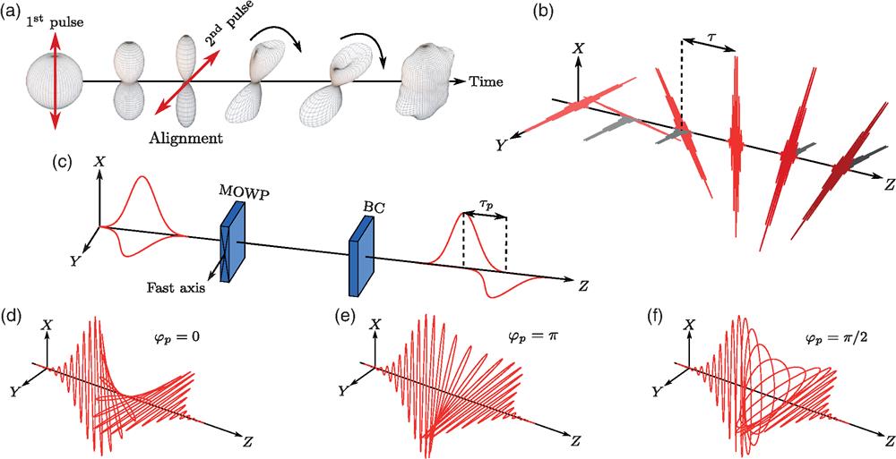
    Fig. 1. Approaches for inducing molecular UDR. (a) Double-pulse scheme for excitation of unidirectional molecular rotation (adapted from Ref. 53, CC BY). (b) A train of linearly polarized laser pulses are spaced in time by a fixed delay τ, and the polarization axis rotates between each pulse.79 (c) Polarization shaping setup. (d), (e) Illustrations of the electric field of the pulse for phase φp=0 and π (2π), producing a linear “twisted” polarization in the clockwise and counterclockwise directions, respectively. (f) The same for intermediate phase φp=π/2, resulting in an elliptical polarization in the region of overlap of the two pulses. Panels (c)–(f) are adapted with permission from Ref. 58, © 2020, American Physical Society (APS).
    Illustration of an optical centrifuge pulse. The vector k denotes the propagation direction of the pulse. The vector of linear polarization E undergoes an accelerated rotation about the propagation direction. (b) Frequency spectra of a full (dashed) and truncated (solid) centrifuge pulse. (c) Time-frequency spectrogram of the centrifuge field, recorded by means of cross-correlation frequency resolved optical gating. This figure is reproduced with permission from Ref. 63, © 2020, APS.
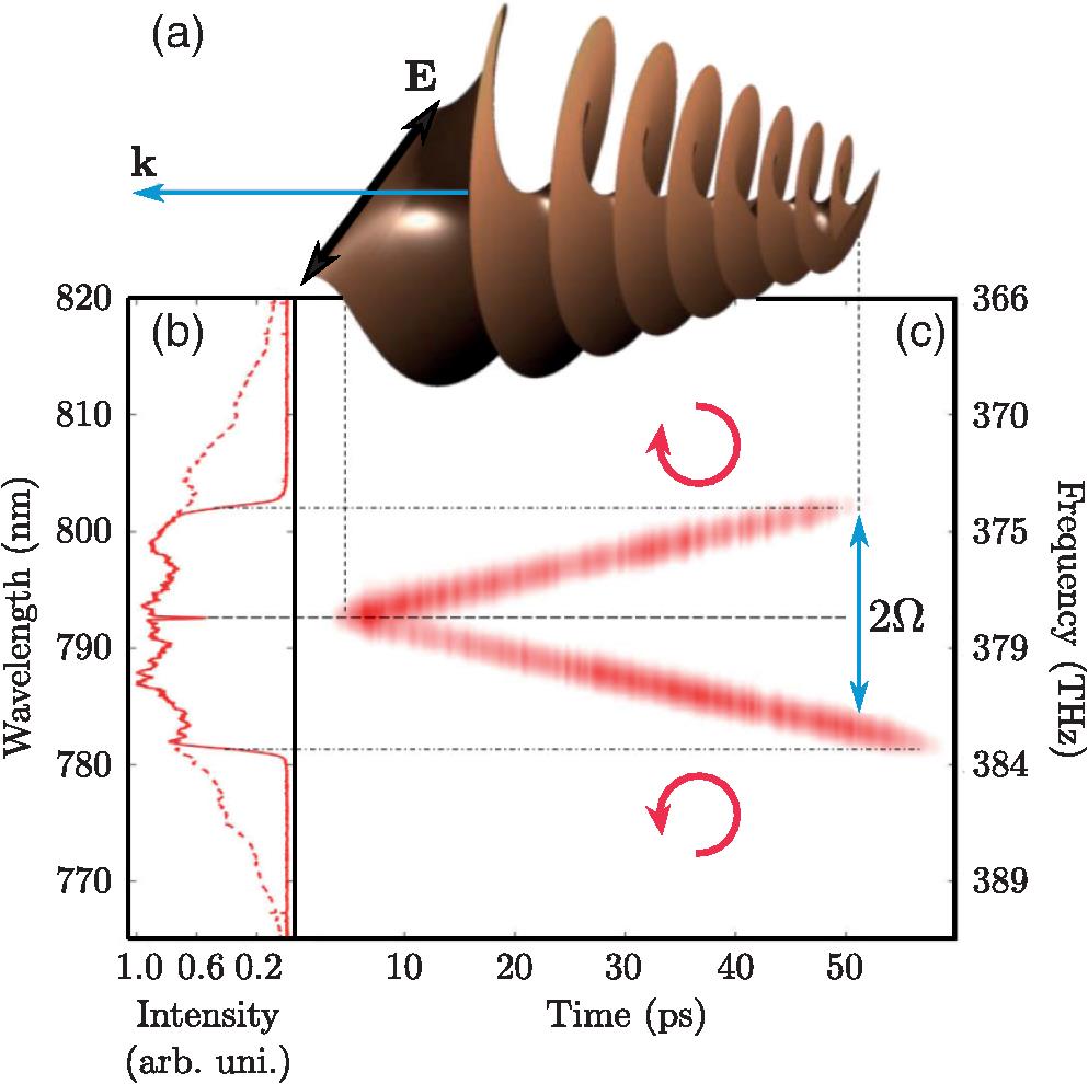
    Fig. 2. Illustration of an optical centrifuge pulse. The vector k denotes the propagation direction of the pulse. The vector of linear polarization E undergoes an accelerated rotation about the propagation direction. (b) Frequency spectra of a full (dashed) and truncated (solid) centrifuge pulse. (c) Time-frequency spectrogram of the centrifuge field, recorded by means of cross-correlation frequency resolved optical gating. This figure is reproduced with permission from Ref. 63, © 2020, APS.
    Experimentally observed RDS for deuterium molecules. (a)–(c) The spectra, shown as 2-D color-coded plots, were measured with a probe scan delay of 150 fs around the midway point between the pump pulses. (d)–(f) Normalized spectra measured at the probe delay time that produced the maximum signal [indicated by the horizontal gray lines in (a)–(c)]. Vertical black line marks the central wavelength of the unperturbed probe. (a), (d) A single pump pulse is applied, resulting in no UDR and no RDS. (b), (e) The molecules are set to rotate in the same sense as the CP probe, producing a red shift. (c), (f) The molecules are set to rotate in the opposite sense, producing a blue shift. This figure is reproduced with permission from Ref. 80.
    Fig. 3. Experimentally observed RDS for deuterium molecules. (a)–(c) The spectra, shown as 2-D color-coded plots, were measured with a probe scan delay of 150 fs around the midway point between the pump pulses. (d)–(f) Normalized spectra measured at the probe delay time that produced the maximum signal [indicated by the horizontal gray lines in (a)–(c)]. Vertical black line marks the central wavelength of the unperturbed probe. (a), (d) A single pump pulse is applied, resulting in no UDR and no RDS. (b), (e) The molecules are set to rotate in the same sense as the CP probe, producing a red shift. (c), (f) The molecules are set to rotate in the opposite sense, producing a blue shift. This figure is reproduced with permission from Ref. 80.
    Time-dependent Raman shifts. From the (a) clockwise and (b) counterclockwise centrifuged oxygen molecules. As the molecules spend more time in the centrifuge, the observed Raman frequency shift increases, providing direct evidence of accelerated molecular rotation in one, well defined, direction. An additional time-independent Raman signal originates from the molecules lost from the centrifuge. This figure is reproduced with permission from Ref. 63, © 2020, APS.
    Fig. 4. Time-dependent Raman shifts. From the (a) clockwise and (b) counterclockwise centrifuged oxygen molecules. As the molecules spend more time in the centrifuge, the observed Raman frequency shift increases, providing direct evidence of accelerated molecular rotation in one, well defined, direction. An additional time-independent Raman signal originates from the molecules lost from the centrifuge. This figure is reproduced with permission from Ref. 63, © 2020, APS.
    COLTRIMS experimental setup for molecular UDR measurements. The measurement is performed in an ultra-high-vacuum apparatus of COLTRIMS. A supersonic gas jet of nitrogen molecules is impulsively aligned by a linearly polarized (along z axis) pulse, which is subsequently kicked to rotate unidirectionally by a properly matched second pulse (polarized at π/4 in the yz plane). An intense circularly polarized probe pulse with adjustable time delay is used to Coulomb explode the molecule allowing the imaging of the evolution of the rotational wave packet. The insets (a)–(f) are the snapshots of the measured momentum distribution of the fragments of the Coulomb exploded nitrogen molecule, and the insets (A)–(F) are the simulated distributions of the rotational wave packet at various time delays. Figure adapted with permission from Ref. 81, © 2020, APS.
    Fig. 5. COLTRIMS experimental setup for molecular UDR measurements. The measurement is performed in an ultra-high-vacuum apparatus of COLTRIMS. A supersonic gas jet of nitrogen molecules is impulsively aligned by a linearly polarized (along z axis) pulse, which is subsequently kicked to rotate unidirectionally by a properly matched second pulse (polarized at π/4 in the yz plane). An intense circularly polarized probe pulse with adjustable time delay is used to Coulomb explode the molecule allowing the imaging of the evolution of the rotational wave packet. The insets (a)–(f) are the snapshots of the measured momentum distribution of the fragments of the Coulomb exploded nitrogen molecule, and the insets (A)–(F) are the simulated distributions of the rotational wave packet at various time delays. Figure adapted with permission from Ref. 81, © 2020, APS.
    Time-dependent angular distributions of UDR molecules. (a) Experimentally measured angular distribution of (N+, N+) fragments in the yz plane (see Fig. 5) ejected from a dissociatively doubly ionized nitrogen molecule as a function of the time delay of the probe pulse. White dashed lines denote the crossed and parallel structures of the angular distribution (see the text). The panel was reproduced with permission from Ref. 81, © 2020, APS. (b) Observed time- and angular-dependent probability, in the rotational wave packet dynamics. Before t=0, molecules are randomly distributed (image from Ref. 82, CC BY-NC 4.0). In (a) and (b), molecules are randomly distributed before t=0. (c) Probability density as a function of the molecular angle and the free propagation time of D2 prepared in the equal-weight superposition of N=2 and N=4 states. The observed nondispersing behavior illustrates the main property of a quantum cogwheel state. The classical period is indicated with the white horizontal bar at the lower right corner. Reproduced from Ref. 105 with permission from the PCCP Owner Societies.
    Fig. 6. Time-dependent angular distributions of UDR molecules. (a) Experimentally measured angular distribution of (N+, N+) fragments in the yz plane (see Fig. 5) ejected from a dissociatively doubly ionized nitrogen molecule as a function of the time delay of the probe pulse. White dashed lines denote the crossed and parallel structures of the angular distribution (see the text). The panel was reproduced with permission from Ref. 81, © 2020, APS. (b) Observed time- and angular-dependent probability, in the rotational wave packet dynamics. Before t=0, molecules are randomly distributed (image from Ref. 82, CC BY-NC 4.0). In (a) and (b), molecules are randomly distributed before t=0. (c) Probability density as a function of the molecular angle and the free propagation time of D2 prepared in the equal-weight superposition of N=2 and N=4 states. The observed nondispersing behavior illustrates the main property of a quantum cogwheel state. The classical period is indicated with the white horizontal bar at the lower right corner. Reproduced from Ref. 105 with permission from the PCCP Owner Societies.
    Field-free enantioselective orientation of PPO molecule. (a) Schematic illustration of the experimental geometry. Cold PPO molecules in a seeded helium jet are spun in an optical centrifuge and Coulomb exploded with a probe pulse between the plates of a conventional VMI spectrometer, equipped with an MCP detector and a phosphor screen. The inset shows the fixed frame axes and the definition of angles θ and θ2-D used in text. (b) (R)-PPO molecule. Atoms are color-coded: black, carbon; gray, hydrogen; and red, oxygen. Principal axes of inertia tensor (I frame) are shown as solid arrows and labeled by a, b, and c (moments of inertia are ordered Ia<Ib<Ic), whereas those of polarizability tensor (A frame) are shown as dashed arrows and labeled by x1, x2, and x3 (principal polarizabilities are ordered α33<α22<α11). Coulomb explosion trajectories from a stationary molecule are shown with thin black and red lines. (c), (d) Experimentally measured degree of 2-D alignment [panel (c)] and orientation [panel (d)] in the velocity distribution of O+. Blue(red) colored markers correspond to the left- (right-)handed enantiomer. The black dashed curves in upper panels show the intensity profile of the centrifuge field in arbitrary units. (e) Binet ellipsoid. Shown in blue are the allowed trajectories of the angular momentum vector. As an example, two trajectories (Ta− and Tc+) are labeled according to the notation used in the text. (f) Experimentally measured 2-D orientation factor in the velocity distribution of O+ fragments as a function of optical centrifuge-probe pulse delay, t. Orange: right handed molecule, (R)-PPO; blue: left handed molecule, (S)-PPO. Note the reversal of colors between the two plots. Panels (a), (b), and (f) are reproduced with permission from Ref. 122. Panels (c) and (d) are reproduced with permission from Ref. 68, © 2020, APS.
    Fig. 7. Field-free enantioselective orientation of PPO molecule. (a) Schematic illustration of the experimental geometry. Cold PPO molecules in a seeded helium jet are spun in an optical centrifuge and Coulomb exploded with a probe pulse between the plates of a conventional VMI spectrometer, equipped with an MCP detector and a phosphor screen. The inset shows the fixed frame axes and the definition of angles θ and θ2-D used in text. (b) (R)-PPO molecule. Atoms are color-coded: black, carbon; gray, hydrogen; and red, oxygen. Principal axes of inertia tensor (I frame) are shown as solid arrows and labeled by a, b, and c (moments of inertia are ordered Ia<Ib<Ic), whereas those of polarizability tensor (A frame) are shown as dashed arrows and labeled by x1, x2, and x3 (principal polarizabilities are ordered α33<α22<α11). Coulomb explosion trajectories from a stationary molecule are shown with thin black and red lines. (c), (d) Experimentally measured degree of 2-D alignment [panel (c)] and orientation [panel (d)] in the velocity distribution of O+. Blue(red) colored markers correspond to the left- (right-)handed enantiomer. The black dashed curves in upper panels show the intensity profile of the centrifuge field in arbitrary units. (e) Binet ellipsoid. Shown in blue are the allowed trajectories of the angular momentum vector. As an example, two trajectories (Ta and Tc+) are labeled according to the notation used in the text. (f) Experimentally measured 2-D orientation factor in the velocity distribution of O+ fragments as a function of optical centrifuge-probe pulse delay, t. Orange: right handed molecule, (R)-PPO; blue: left handed molecule, (S)-PPO. Note the reversal of colors between the two plots. Panels (a), (b), and (f) are reproduced with permission from Ref. 122. Panels (c) and (d) are reproduced with permission from Ref. 68, © 2020, APS.
    Trajectories of the polarization vector tip of the OTC pulse in case (a) when the amplitude of the FW is greater than that of the SH and (b) vice versa. (c) Optical layout for constructing a collinearly propagating two-color field by nonlinear optical-mixing technique. MPA, most polarizable axis and SMPA, second most polarizable axis. Notice that in case of SO2 SMPA is the axis that must be oriented, whereas in case of iodobenzene MPA is the one requiring orientation. Panel (c) is adapted with permission from Ref. 152, © 2020, APS.
    Fig. 8. Trajectories of the polarization vector tip of the OTC pulse in case (a) when the amplitude of the FW is greater than that of the SH and (b) vice versa. (c) Optical layout for constructing a collinearly propagating two-color field by nonlinear optical-mixing technique. MPA, most polarizable axis and SMPA, second most polarizable axis. Notice that in case of SO2 SMPA is the axis that must be oriented, whereas in case of iodobenzene MPA is the one requiring orientation. Panel (c) is adapted with permission from Ref. 152, © 2020, APS.
    1-D model describing the OTC pulse-induced orientation. (a) SO2 molecule, the atoms are color coded: sulfur, yellow and oxygen, red. The major axis is perfectly aligned along the laboratory Y axis. The minor axis lies in the XZ plane at an angle θ relative to the Z axis. (b) Potential energy as a function of θ for ϕL=0,π,π/2, [see Eqs. (3) and (4)]. This figure is from Ref. 146, CC BY 4.0.
    Fig. 9. 1-D model describing the OTC pulse-induced orientation. (a) SO2 molecule, the atoms are color coded: sulfur, yellow and oxygen, red. The major axis is perfectly aligned along the laboratory Y axis. The minor axis lies in the XZ plane at an angle θ relative to the Z axis. (b) Potential energy as a function of θ for ϕL=0,π,π/2, [see Eqs. (3) and (4)]. This figure is from Ref. 146, CC BY 4.0.
    Coincidentally measured momentum distributions of S+ (vertical panels) and O+ (horizontal panels). Here pY and pZ are the projections of fragments’ momenta on Y and Z axes, respectively (measured in atomic units). (a) Isotropic momentum distribution for S+ and O+ ions measured before the arrival of OTC pulse. (b), (c) Anisotropic momentum distributions for S+ and O+ ions measured at t≈0.2 ps after the application of the OTC pulse at ϕL=0 and π, respectively. (d), (e) Angular distributions of ϕSY derived from (b) and (c), respectively. Gray bars represent the uncertainty propagated during data analysis according to Gaussian’ s propagation law. This figure is from Ref. 146, CC BY 4.0.
    Fig. 10. Coincidentally measured momentum distributions of S+ (vertical panels) and O+ (horizontal panels). Here pY and pZ are the projections of fragments’ momenta on Y and Z axes, respectively (measured in atomic units). (a) Isotropic momentum distribution for S+ and O+ ions measured before the arrival of OTC pulse. (b), (c) Anisotropic momentum distributions for S+ and O+ ions measured at t0.2  ps after the application of the OTC pulse at ϕL=0 and π, respectively. (d), (e) Angular distributions of ϕSY derived from (b) and (c), respectively. Gray bars represent the uncertainty propagated during data analysis according to Gaussian’ s propagation law. This figure is from Ref. 146, CC BY 4.0.
    A sequence of two short-orienting pulses (P1,P2) is applied. The pulses are delayed by the time T. After an additional delay that is after 2T, an impulsive response emerges, denoted E1. Higher order echoes appear after 3T,4T… This figure is adapted with permission from Ref. 36, © 2020, APS.
    Fig. 11. A sequence of two short-orienting pulses (P1,P2) is applied. The pulses are delayed by the time T. After an additional delay that is after 2T, an impulsive response emerges, denoted E1. Higher order echoes appear after 3T,4T This figure is adapted with permission from Ref. 36, © 2020, APS.
    Filamentation of the phase-space density distribution. In this figure, Ω1/σ=1. (a) Initial smooth phase space distribution (b) shortly after the kick, σt=0.5, the density distribution folds, resulting in a transient alignment along the direction θ=0. The folded pattern is centrally symmetric with respect to the phase-space point (θ,ω)=(0,0) that is not affected by the kick. (c) On the longer time scale, σt=5, the probability density becomes wrinkled and develops multiple parallel filaments. (d) After a second kick is applied at T (with σT=5 and Ω2/Ω1=1/3), every filament in (c) folds in a manner similar to (b), giving rise to an alignment echo near θ=0 at time τ≈T after the second kick (στ=4.56). (e) At τ≈T/2 (στ=2.29), a fractional echo is formed. t refers to time counted from the first pulse, whereas τ to time counted from the second pulse. For details, see Ref. 37.
    Fig. 12. Filamentation of the phase-space density distribution. In this figure, Ω1/σ=1. (a) Initial smooth phase space distribution (b) shortly after the kick, σt=0.5, the density distribution folds, resulting in a transient alignment along the direction θ=0. The folded pattern is centrally symmetric with respect to the phase-space point (θ,ω)=(0,0) that is not affected by the kick. (c) On the longer time scale, σt=5, the probability density becomes wrinkled and develops multiple parallel filaments. (d) After a second kick is applied at T (with σT=5 and Ω2/Ω1=1/3), every filament in (c) folds in a manner similar to (b), giving rise to an alignment echo near θ=0 at time τT after the second kick (στ=4.56). (e) At τT/2 (στ=2.29), a fractional echo is formed. t refers to time counted from the first pulse, whereas τ to time counted from the second pulse. For details, see Ref. 37.
    Left: Hahn’s famous spin echo analogy on the cover of Physics Today (Ref. 167). Pictorial rotational density matrix representations of (a) an effective two level system invoked by the Raman selection rule (ΔJ=±2). (b) Two coherent pathways starting from a mutual population term |J⟩⟨J| and interfere to create the rephasing coherence term |J+2⟩⟨J|. (c) Two coherent pathways starting from two neighboring population terms |J⟩⟨J| and |J+2⟩⟨J+2| that interfere at the rephasing coherence term |J+2⟩⟨J|. This figure is reproduced with permission from Ref. 168, © 2020, APS.
    Fig. 13. Left: Hahn’s famous spin echo analogy on the cover of Physics Today (Ref. 167). Pictorial rotational density matrix representations of (a) an effective two level system invoked by the Raman selection rule (ΔJ=±2). (b) Two coherent pathways starting from a mutual population term |JJ| and interfere to create the rephasing coherence term |J+2J|. (c) Two coherent pathways starting from two neighboring population terms |JJ| and |J+2J+2| that interfere at the rephasing coherence term |J+2J|. This figure is reproduced with permission from Ref. 168, © 2020, APS.
    Left: (a) Birefringence signals as a function of the pump–probe delay τ for intensities I1=38 TW/cm2 and I2=15 TW/cm2 of the pump pulses P1 and P2, respectively, (see the inset). Trev, rotational revival time. (b) Third-harmonic signal detected by selecting the harmonic field component parallel to the alignment axis z. The delay T between P1 and P2 is set to 2.5 ps. Middle: time-dependent angular distributions of full, 1/2 and 1/3 echoes, as indicated between the white dashed lines in (c) 2.2 to 3.5 ps, (f) 1.9 to 3.0 ps, and (i) 1.4 to 1.9 ps, experimentally measured and theoretically simulated for CO2. (c) Carpet of the angular distribution of full echo for parallel input pulses, P1 and P2, with T=3 ps time delay between them. (d), (e) Polar plots of the alignment and antialignment regions of the distribution for the full echo, showing vertical and horizontal directionality, respectively. (f)–(h) The same, for the 1/2 fractional echo, with T=5 ps time delay. (i)–(k) The same for 1/3 fractional echoes with T=5 ps time delay. In all cases, the solid red line is the quantum-mechanically simulated distribution. Panels (a) and (b) are reproduced with permission from Refs. 36 and 38, respectively. Panels (c)–(k) are from Ref. 37 (CC BY 3.0).
    Fig. 14. Left: (a) Birefringence signals as a function of the pump–probe delay τ for intensities I1=38  TW/cm2 and I2=15  TW/cm2 of the pump pulses P1 and P2, respectively, (see the inset). Trev, rotational revival time. (b) Third-harmonic signal detected by selecting the harmonic field component parallel to the alignment axis z. The delay T between P1 and P2 is set to 2.5 ps. Middle: time-dependent angular distributions of full, 1/2 and 1/3 echoes, as indicated between the white dashed lines in (c) 2.2 to 3.5 ps, (f) 1.9 to 3.0 ps, and (i) 1.4 to 1.9 ps, experimentally measured and theoretically simulated for CO2. (c) Carpet of the angular distribution of full echo for parallel input pulses, P1 and P2, with T=3  ps time delay between them. (d), (e) Polar plots of the alignment and antialignment regions of the distribution for the full echo, showing vertical and horizontal directionality, respectively. (f)–(h) The same, for the 1/2 fractional echo, with T=5  ps time delay. (i)–(k) The same for 1/3 fractional echoes with T=5  ps time delay. In all cases, the solid red line is the quantum-mechanically simulated distribution. Panels (a) and (b) are reproduced with permission from Refs. 36 and 38, respectively. Panels (c)–(k) are from Ref. 37 (CC BY 3.0).
    Experimentally measured time-dependent angular distributions of the rotated echo in CO2. P1 and P2 arrive at −3 and 0 ps, respectively, with a relative angle β=π/8. (a) Angular distribution of the rotated echo as a function of the probe time delay (see the region of 2.2 to 3.5 ps between the white dashed lines). (b) Polar plot of the rotated echo at 3 ps. (c), (d) Experimentally measured time-dependent angular distributions of the imaginary echo in CO2. P1 and P2 arrive at −2.6 and 0 ps, respectively. (c) A “carpet” describing the angular distribution of the imaginary echo as a function of the probe time delay (see the region of 36 to 38 ps between the white dashed lines). (d) The alignment factor ⟨cos2 θ⟩ as a function of the probe delay (red shows the revival of the response to the first pulse, blue that of the second pulse, green depicts the revival of the first full echo, and purple presents the imaginary echo). This figure is from Ref. 37, CC BY 3.0.
    Fig. 15. Experimentally measured time-dependent angular distributions of the rotated echo in CO2. P1 and P2 arrive at 3 and 0 ps, respectively, with a relative angle β=π/8. (a) Angular distribution of the rotated echo as a function of the probe time delay (see the region of 2.2 to 3.5 ps between the white dashed lines). (b) Polar plot of the rotated echo at 3 ps. (c), (d) Experimentally measured time-dependent angular distributions of the imaginary echo in CO2. P1 and P2 arrive at 2.6 and 0 ps, respectively. (c) A “carpet” describing the angular distribution of the imaginary echo as a function of the probe time delay (see the region of 36 to 38 ps between the white dashed lines). (d) The alignment factor cos2θ as a function of the probe delay (red shows the revival of the response to the first pulse, blue that of the second pulse, green depicts the revival of the first full echo, and purple presents the imaginary echo). This figure is from Ref. 37, CC BY 3.0.
    (a) Experimental results of the maximal echo amplitude (Sechomax, marked by blue circles), obtained at various delays between pulses, and the corresponding optimal P2 intensities (P2opt, green dots) required to induce them. Theoretical simulations of Sechomax and of P2opt are depicted by the blue triangles (connected by blue dashed curve) and by the green curve, respectively. Note that the x axis depicts the time of the second pulse (Δt), and thus the echo signals (with their maximal amplitudes marked by the blue circles) are observed at 2Δt. (b) Low-pressure temporal traces of the echo recorded in CO2 for different time delays τ12 between the pulse P1 and P2 as a function of the probe delay τ defined with respect to P1. The intensity of P2 is set to the optimal value for the delay τ12=2.4 ps, i.e., 13 TW/cm2. (c) High-pressure temporal traces in CO2−He gas mixture at a pressure of 43.5 bar with an enlargement of the echo decay shown in the inset. The estimated intensity of P1 is 20 TW/cm2. The positions of the alignment peaks respective to P1 and P2 are marked with arrows. (d) Peak-to-dip amplitude of the echo (filled circles) recorded in a CO2−He gas mixture (P=43.5 bar) as a function of τ12 compared with classical molecular dynamics simulations (CMDS) (dashed line). Least squares fitting of the experimental data with an exponential law (solid line). (e) Decay rates γ of the echo (filled circles) measured for various densities of the gas mixture with the linear fit (solid line) of the data and the CMDS calculations (dashed line). The error bars reflect the dispersion of the measurements. The bottom (top) x axis denotes the gas density (pressure) in units of amagat (bar). Panel (a) is reproduced with permission from Ref. 168. Panels (c)–(f) are reproduced with permission from Ref. 174, © 2020, APS.
    Fig. 16. (a) Experimental results of the maximal echo amplitude (Sechomax, marked by blue circles), obtained at various delays between pulses, and the corresponding optimal P2 intensities (P2opt, green dots) required to induce them. Theoretical simulations of Sechomax and of P2opt are depicted by the blue triangles (connected by blue dashed curve) and by the green curve, respectively. Note that the x axis depicts the time of the second pulse (Δt), and thus the echo signals (with their maximal amplitudes marked by the blue circles) are observed at 2Δt. (b) Low-pressure temporal traces of the echo recorded in CO2 for different time delays τ12 between the pulse P1 and P2 as a function of the probe delay τ defined with respect to P1. The intensity of P2 is set to the optimal value for the delay τ12=2.4  ps, i.e., 13  TW/cm2. (c) High-pressure temporal traces in CO2He gas mixture at a pressure of 43.5 bar with an enlargement of the echo decay shown in the inset. The estimated intensity of P1 is 20  TW/cm2. The positions of the alignment peaks respective to P1 and P2 are marked with arrows. (d) Peak-to-dip amplitude of the echo (filled circles) recorded in a CO2He gas mixture (P=43.5 bar) as a function of τ12 compared with classical molecular dynamics simulations (CMDS) (dashed line). Least squares fitting of the experimental data with an exponential law (solid line). (e) Decay rates γ of the echo (filled circles) measured for various densities of the gas mixture with the linear fit (solid line) of the data and the CMDS calculations (dashed line). The error bars reflect the dispersion of the measurements. The bottom (top) x axis denotes the gas density (pressure) in units of amagat (bar). Panel (a) is reproduced with permission from Ref. 168. Panels (c)–(f) are reproduced with permission from Ref. 174, © 2020, APS.
    Time constants of collisional relaxation of N2O. The circles with error bars (representing two standard deviations of the mean) are the density-normalized decay time constants τE of the echoes deduced from the measurements of the alignment signal recorded at various N2O(4%)+He(96%) gas densities and fixed delays τ12 between the two pulses. The dashed lines denote the results of simulations conducted by solving the density matrix equations for molecules impulsively aligned by two short laser pulses and interacting with each other through collisions. The red dashed lines have been obtained using the standard Bloch equations (i.e., using the secular approximation) and the green dashed line represents the results obtained using the nonsecular Redfield equations. This figure is adapted from Ref. 175 (CC BY 4.0).
    Fig. 17. Time constants of collisional relaxation of N2O. The circles with error bars (representing two standard deviations of the mean) are the density-normalized decay time constants τE of the echoes deduced from the measurements of the alignment signal recorded at various N2O(4%)+He(96%) gas densities and fixed delays τ12 between the two pulses. The dashed lines denote the results of simulations conducted by solving the density matrix equations for molecules impulsively aligned by two short laser pulses and interacting with each other through collisions. The red dashed lines have been obtained using the standard Bloch equations (i.e., using the secular approximation) and the green dashed line represents the results obtained using the nonsecular Redfield equations. This figure is adapted from Ref. 175 (CC BY 4.0).
    Kang Lin, Ilia Tutunnikov, Junyang Ma, Junjie Qiang, Lianrong Zhou, Olivier Faucher, Yehiam Prior, Ilya Sh. Averbukh, Jian Wu. Spatiotemporal rotational dynamics of laser-driven molecules[J]. Advanced Photonics, 2020, 2(2): 024002
    Download Citation