• Photonics Research
  • Vol. 9, Issue 3, B71 (2021)
Xianxin Guo1、2、3、5、†,*, Thomas D. Barrett2、6、†,*, Zhiming M. Wang1、7、*, and A. I. Lvovsky2、4、8、*
Author Affiliations
  • 1Institute of Fundamental and Frontier Sciences, University of Electronic Science and Technology of China, Chengdu 610054, China
  • 2Clarendon Laboratory, University of Oxford, Oxford OX1 3PU, UK
  • 3Institute for Quantum Science and Technology, University of Calgary, Calgary, Alberta T2N 1N4, Canada
  • 4Russian Quantum Center, Skolkovo 143025, Moscow, Russia
  • 5e-mail: xianxin.guo@physics.ox.ac.uk
  • 6e-mail: thomas.barrett@physics.ox.ac.uk
  • 7e-mail: zhmwang@uestc.edu.cn
  • 8e-mail: alex.lvovsky@physics.ox.ac.uk
  • show less
    DOI: 10.1364/PRJ.411104 Cite this Article Set citation alerts
    Xianxin Guo, Thomas D. Barrett, Zhiming M. Wang, A. I. Lvovsky. Backpropagation through nonlinear units for the all-optical training of neural networks[J]. Photonics Research, 2021, 9(3): B71 Copy Citation Text show less
    ONN with all-optical forward- and backward-propagation. (a) A single ONN layer that consists of weighted interconnections and an SA nonlinear activation function. The forward- (red) and backward-propagating (orange) optical signals, whose amplitudes are proportional to the neuron activations, a(l−1), and errors, δ(l), respectively, are tapped off by beam splitters, measured by heterodyne detection and multiplied to determine the weight matrix update in Eq. (2). This multiplication can also be implemented optically, as discussed in the text. The final update of the weights, as well as the preparation of network input, is implemented electronically. (b) Error calculation at the output layer performed optically or digitally, as described in the text.
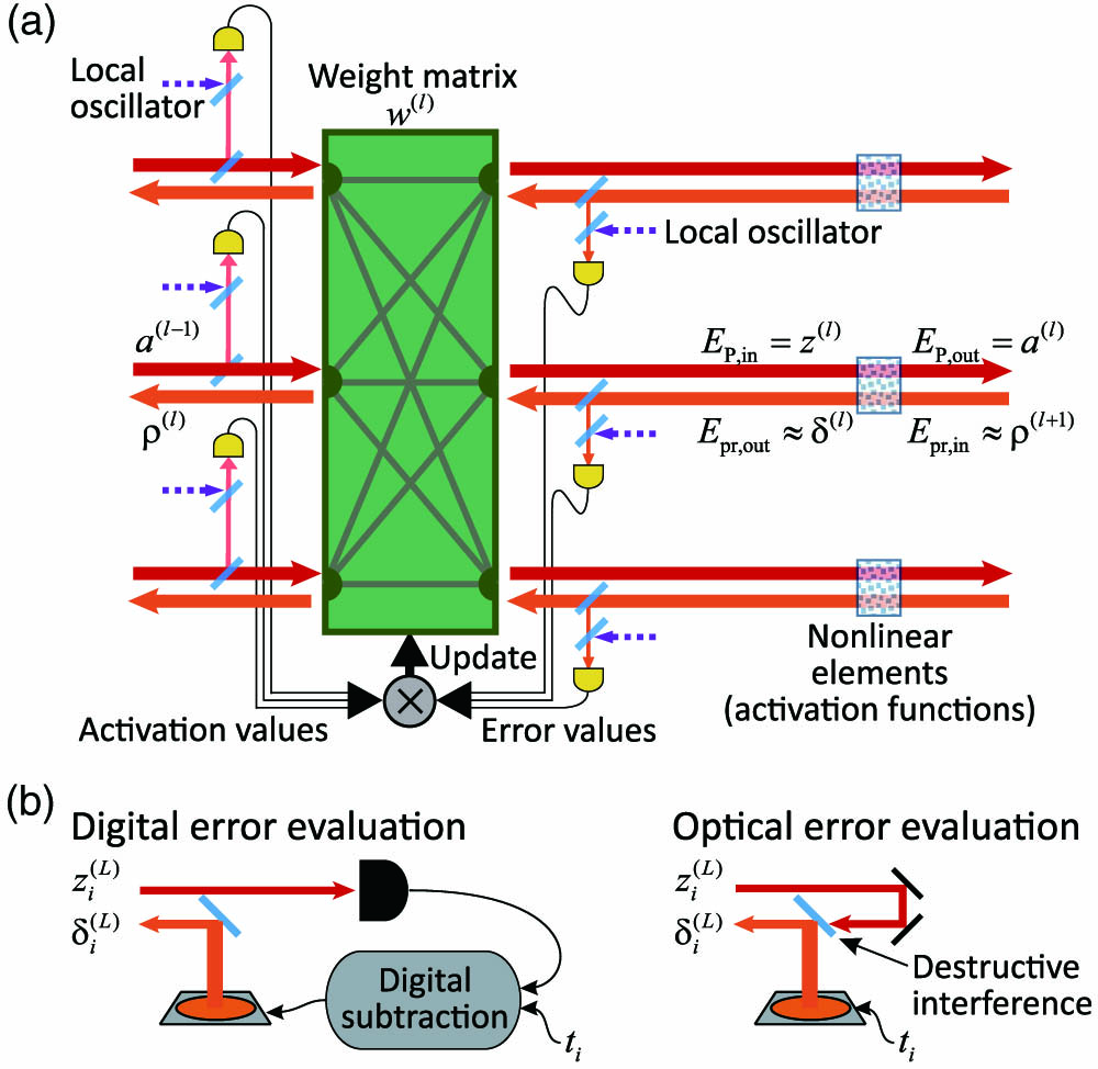
    Fig. 1. ONN with all-optical forward- and backward-propagation. (a) A single ONN layer that consists of weighted interconnections and an SA nonlinear activation function. The forward- (red) and backward-propagating (orange) optical signals, whose amplitudes are proportional to the neuron activations, a(l1), and errors, δ(l), respectively, are tapped off by beam splitters, measured by heterodyne detection and multiplied to determine the weight matrix update in Eq. (2). This multiplication can also be implemented optically, as discussed in the text. The final update of the weights, as well as the preparation of network input, is implemented electronically. (b) Error calculation at the output layer performed optically or digitally, as described in the text.
    Saturable absorber response. (a) The transmission and (b) transmission derivative of an SA unit with optical depths of 1 (left) and 30 (right), as defined by Eqs. (4) and (6), respectively. Also shown in panel (b) are the actual probe transmissions given by Eq. (5), which approximate the derivatives, with and without the rescaling. The scaling factors are 1.2 (left) and 2.5 (right). In the amplitude region (i), the SA behaves as a linear absorber for weak input but then exhibits strong nonlinearity when the pump intensity approaches the saturation threshold. Region (ii) corresponds to strong saturation: the ground-state population is depleted, and the absorber is rendered transparent.
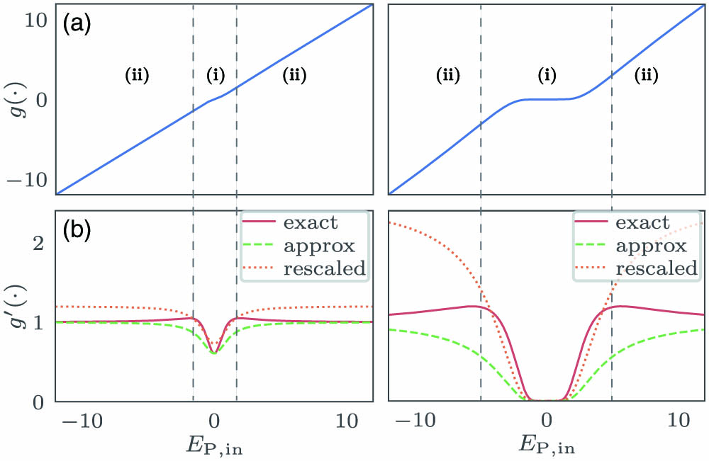
    Fig. 2. Saturable absorber response. (a) The transmission and (b) transmission derivative of an SA unit with optical depths of 1 (left) and 30 (right), as defined by Eqs. (4) and (6), respectively. Also shown in panel (b) are the actual probe transmissions given by Eq. (5), which approximate the derivatives, with and without the rescaling. The scaling factors are 1.2 (left) and 2.5 (right). In the amplitude region (i), the SA behaves as a linear absorber for weak input but then exhibits strong nonlinearity when the pump intensity approaches the saturation threshold. Region (ii) corresponds to strong saturation: the ground-state population is depleted, and the absorber is rendered transparent.
    Effects of imperfect approximation of the activation function derivative. (a) Feed-forward neural network architecture using a single hidden layer of 128 neurons. (b) Distribution of neuron inputs (EP,in(1)≡z(1)), which is concentrated in the unsaturated region (1) of the SA activation function, g(·). As a result, the approximation error in the linear region (2) is less impactful on the training. (c) The transmission of an SA unit with α0=10, along with the exact and (rescaled for easier comparison) optically approximated transmission derivatives. (d) Performance loss associated with approximating activation function derivatives g′(·) with random functions, plotted as a function of the approximation error, for α0=10 (see Appendix B for details). (e) Average error of the derivative approximation in Eq. (5) as a function of the optical depth of an SA nonlinearity.
    Fig. 3. Effects of imperfect approximation of the activation function derivative. (a) Feed-forward neural network architecture using a single hidden layer of 128 neurons. (b) Distribution of neuron inputs (EP,in(1)z(1)), which is concentrated in the unsaturated region (1) of the SA activation function, g(·). As a result, the approximation error in the linear region (2) is less impactful on the training. (c) The transmission of an SA unit with α0=10, along with the exact and (rescaled for easier comparison) optically approximated transmission derivatives. (d) Performance loss associated with approximating activation function derivatives g(·) with random functions, plotted as a function of the approximation error, for α0=10 (see Appendix B for details). (e) Average error of the derivative approximation in Eq. (5) as a function of the optical depth of an SA nonlinearity.
    Performance on image classification. (a) (i) The fully connected network architecture. (ii) Learning curves for the SA [with either exact derivatives in Eq. (6) of the activation function or their approximation in Eq. (5)] and benchmark ReLU networks. (iii) The final classification accuracy achieved as a function of the optical depth, α0, of the SA cell. (b) (i) The convolutional network architecture. Sequential convolution layers of 32 and 64 channels convert a 28×28 pixel image into a 1024-dimensional feature vector, which is then classified (into NC=10 classes for MNIST and KMNIST, and NC=47 classes for EMNIST) by fully connected layers. Pooling layers are not shown for simplicity. (ii) Classification accuracy of convolutional networks when using various activation functions. The same deep network architecture is applied to all data sets, but the SA networks use mean-pooling, while the benchmark networks use max-pooling. The last row shows the performance of a simple linear classifier as a baseline.
    Fig. 4. Performance on image classification. (a) (i) The fully connected network architecture. (ii) Learning curves for the SA [with either exact derivatives in Eq. (6) of the activation function or their approximation in Eq. (5)] and benchmark ReLU networks. (iii) The final classification accuracy achieved as a function of the optical depth, α0, of the SA cell. (b) (i) The convolutional network architecture. Sequential convolution layers of 32 and 64 channels convert a 28×28 pixel image into a 1024-dimensional feature vector, which is then classified (into NC=10 classes for MNIST and KMNIST, and NC=47 classes for EMNIST) by fully connected layers. Pooling layers are not shown for simplicity. (ii) Classification accuracy of convolutional networks when using various activation functions. The same deep network architecture is applied to all data sets, but the SA networks use mean-pooling, while the benchmark networks use max-pooling. The last row shows the performance of a simple linear classifier as a baseline.
    Optical backpropagation through saturable gain (SG) nonlinearity. (a) Fully connected network architecture, which is the same as Fig. 4(a) except for the nonlinearity. (b) Transmission and transmission derivatives of the SG unit with gain factor g0=3. (c) Learning curves for the SG-based ONN and benchmark ReLU networks. (d) The final classification accuracy achieved as a function of the gain.
    Fig. 5. Optical backpropagation through saturable gain (SG) nonlinearity. (a) Fully connected network architecture, which is the same as Fig. 4(a) except for the nonlinearity. (b) Transmission and transmission derivatives of the SG unit with gain factor g0=3. (c) Learning curves for the SG-based ONN and benchmark ReLU networks. (d) The final classification accuracy achieved as a function of the gain.
    Xianxin Guo, Thomas D. Barrett, Zhiming M. Wang, A. I. Lvovsky. Backpropagation through nonlinear units for the all-optical training of neural networks[J]. Photonics Research, 2021, 9(3): B71
    Download Citation