Xianxin Guo, Thomas D. Barrett, Zhiming M. Wang, A. I. Lvovsky, "Backpropagation through nonlinear units for the all-optical training of neural networks," Photonics Res. 9, B71 (2021)
Copy Citation Text
We propose a practical scheme for end-to-end optical backpropagation in neural networks. Using saturable absorption for the nonlinear units, we find that the backward-propagating gradients required to train the network can be approximated in a surprisingly simple pump-probe scheme that requires only simple passive optical elements. Simulations show that, with readily obtainable optical depths, our approach can achieve equivalent performance to state-of-the-art computational networks on image classification benchmarks, even in deep networks with multiple sequential gradient approximation. With backpropagation through nonlinear units being an outstanding challenge to the field, this work provides a feasible path toward truly all-optical neural networks.
1. INTRODUCTION
Machine learning (ML) is changing the way in which we approach complex tasks, with applications ranging from natural language processing [1] and image recognition [2] to artificial intelligence [3] and fundamental science [4,5]. At the heart (or “brain”) of this revolution are artificial neural networks (ANNs), which are universal function approximators [6,7] capable, in principle, of representing an arbitrary mapping of inputs to outputs. Remarkably, their function only requires two basic operations: matrix multiplication to communicate information between layers, and some nonlinear transformation of individual neuron states (activation function). The former accounts for most of the computational cost associated with ML. This operation can, however, be readily implemented by leveraging the coherence and superposition properties of linear optics [8]. Optics is therefore an attractive platform for realizing the next generation of neural networks, promising faster computation with low power consumption [9–13].
Proposals for optical neural networks (ONNs) have been around for over 30 years [14,15] and have been realized in both free-space [16–18] and integrated [9,10] settings. However, the true power of neural networks is not only that they can approximate arbitrary functions, but also that they can “learn” that approximation. The training of neural networks is, almost universally, achieved by the backpropagation algorithm [19]. Implementing this algorithm optically is challenging because it requires the response of the network’s nonlinear elements to be different for light propagating forward or backward. Confronted with these challenges, existing ONNs are actually trained with, or heavily aided by, digital computers [9,16,18,20]. As a result, the great advantages offered by optics remain largely unexploited. Developing an all-optically trained ONN to leverage these advantages remains an unsolved problem. Here, we address this challenge and present a practical training method capable of backpropagating the error signal through nonlinear neurons in a single optical pass.
The backpropagation algorithm aims to minimize a loss function that quantifies the divergence of the network’s current performance from the ideal, via gradient descent [19]. To do so, the following steps are repeated until convergence: (1) forward propagation of information through the network; (2) evaluation of the loss function gradients with respect to the network parameters at the output layer; (3) backpropagation of these gradients to all previous layers; (4) parameter updates in the direction that maximally reduces the loss function. Forward propagation [step (1)] requires the aforementioned matrix multiplication, which maps information between layers, and a suitable nonlinear activation function, which is applied individually to each neuron. While this nonlinearity has so far been mostly applied digitally in hybrid optical-electronic systems [9,20–22]—at the cost of repeatedly measuring and generating the optical state—recent work has also realized optical nonlinearities [18,23–25].
Sign up for Photonics Research TOC. Get the latest issue of Photonics Research delivered right to you!Sign up now
However, obtaining and backpropagating the loss-function gradients [(steps (2) and (3)] remains an outstanding problem in an optical setting. While backpropagating through the linear interconnection between layers is rather straightforward, as linear optical operations are naturally bidirectional, the nonlinearity of neurons is a challenge. This is because the backward-propagating signal must be modulated by the derivatives of the activation function of each neuron at its current input value, and these derivatives are not readily available in an ONN.
In 1987, Wagner et al. suggested that a feedforward ONN could be implemented and trained by using Fabry–Perot etalons to approximate the required forward and backward response of a sigmoid nonlinearity [26]. However, this backpropagation approach was never realized or even analyzed in detail, largely due to its inherent experimental complexity, with a subsequent ONN demonstration instead using digitally calculated errors [27]. A further approach to an optically trained feedforward network was proposed by Cruz-Cabrera et al. [28]. The authors used a highly nonstandard network architecture that transforms a “continuum of neurons” (a wavefront) as it passes through a nonlinear crystal using cross-phase modulation with a secondary “weight” beam. In a proof-of-concept experiment, the learning of two-bit logic was demonstrated.
An additional challenge is to map from the gradients with respect to the (platform-agnostic) weight matrices to the physical parameters that control these matrices in a specific ONN platform. In 2018, Hughes et al. [20] proposed a method to directly obtain the gradients of these control parameters by an additional forward-propagating step. However, this scheme assumes computing the derivatives of the activation functions digitally and applying them to the backpropagating signal electro-optically.
This work directly addresses the issue of optical backpropagation through nonlinear units in a manner that is both consistent with modern neural network architectures and compatible with leading ONN designs [9,20,29,30]. We consider an optical nonlinearity based on saturable absorption (SA) and show that, with the forward-propagating features and the backward-propagating errors taking the roles of pump and probe, respectively, backpropagation can be realized using only passive optical elements. Our method is effective and surprisingly simple, with the required optical operations for both forward and backward propagation realized using the same physical elements. Simulations with physically realistic parameters show that the proposed scheme can train networks to performance levels equivalent to state-of-the-art ANNs. When combined with optical calculation of the error term at the output layer via interference, this presents a path to the all-optical training of ONNs.
2. IMPLEMENTING OPTICAL BACKPROPAGATION
We begin by recapping the operation of a neural network before discussing optical implementations. Seeded with data at the input layer (), forward-propagation maps the neuron activations from layer to the neuron inputs at layer as via a weight matrix , before applying a nonlinear activation function individually to each neuron, (with subscripts labelling individual neurons).
At the output layer, we evaluate the loss function, , and calculate its gradient with respect to the weights, where is commonly referred to as the “error” at the th neuron in the th layer. From the chain rule, we have where . Given the error at the output layer, i.e., , which is calculated directly from the loss function, the errors for all preceding layers are sequentially found using Eq. (3). These errors, as well as the activations of all neurons, allow one to find the gradients [Eq. (2)] of the error function with respect to all the weights and hence apply the gradient descent.
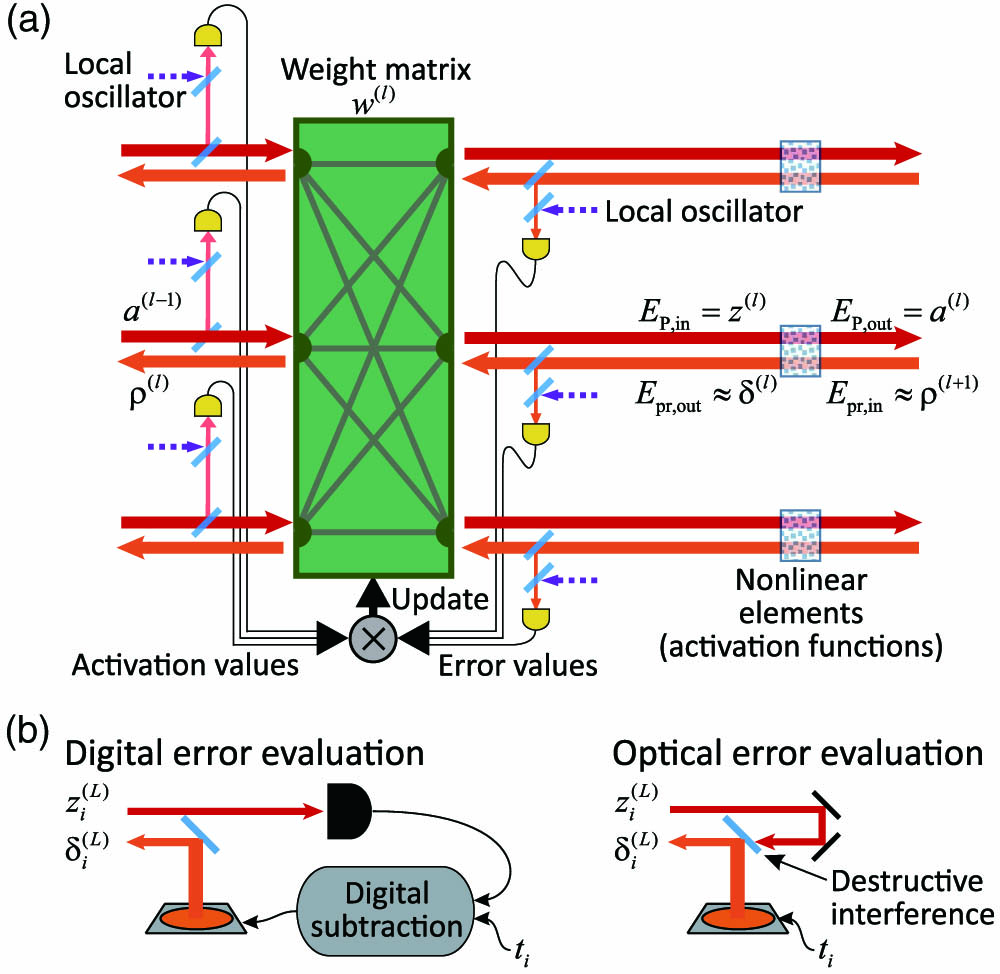
Figure 1.ONN with all-optical forward- and backward-propagation. (a) A single ONN layer that consists of weighted interconnections and an SA nonlinear activation function. The forward- (red) and backward-propagating (orange) optical signals, whose amplitudes are proportional to the neuron activations, , and errors, , respectively, are tapped off by beam splitters, measured by heterodyne detection and multiplied to determine the weight matrix update in Eq. (2). This multiplication can also be implemented optically, as discussed in the text. The final update of the weights, as well as the preparation of network input, is implemented electronically. (b) Error calculation at the output layer performed optically or digitally, as described in the text.
To address this challenge, we require an optical implementation of the activation function with the following features: (i) nonlinear response for the forward input; (ii) linear response for the backward input; (iii) modulation of backward input with the derivative of the nonlinear function. While it is natural to use nonlinear optics for this purpose, it is difficult to satisfy the requirement that the unit must respond differently to forward- and backward-propagating light. Here, we show that this problem can be addressed using saturable absorption in the well-known pump-probe configuration.
Figure 2.Saturable absorber response. (a) The transmission and (b) transmission derivative of an SA unit with optical depths of 1 (left) and 30 (right), as defined by Eqs. (4) and (6), respectively. Also shown in panel (b) are the actual probe transmissions given by Eq. (5), which approximate the derivatives, with and without the rescaling. The scaling factors are 1.2 (left) and 2.5 (right). In the amplitude region (i), the SA behaves as a linear absorber for weak input but then exhibits strong nonlinearity when the pump intensity approaches the saturation threshold. Region (ii) corresponds to strong saturation: the ground-state population is depleted, and the absorber is rendered transparent.
Note that both beams are assumed to be resonant with the atomic transition and so, as the phase of the electric field is unchanged, we treat these as real-valued without loss of generality. Therefore, with the pump and probe taking the roles of the forward-propagating signal and backward-propagating error in an ONN, required features (i) and (ii) of our optical nonlinear unit are met.
Condition (iii), however, remains to be satisfied. The derivative of the pump transmission is
The derivatives at of 1 and 30 are plotted in Fig. 2(b). Our key insight is that, in many instances, the square-bracketed factor in Eq. (6) can be considered constant, in which case the backpropagation transmission of Eq. (5) is a good approximation of the desired response in Eq. (6) up to a constant factor. Feature (iii) is then satisfied because a constant scaling of the network gradients can be absorbed into the learning rate. This may appear as a coarse approximation, however; as we will see in the next section, it is only required to hold within the nonlinear region of the SA response, which is the case for our system [Fig. 2(b)].
The proposed scheme can be implemented on either integrated or free-space platforms. In the integrated setting, optical interference units that combine integrated phase-shifters and attenuators to realize intralayer weights have been demonstrated [9] as have, separately, on-chip SA through atomic vapor [32,33] and other nonlinear media [23,34]. A free-space implementation of the required matrix multiplication can be achieved using a spatial light modulator (SLM) [8,31] with the nonlinear unit provided by a standard atomic vapor cell. In the integrated case, an additional nontrivial step to map the weight gradients in Eq. (2) to suitable updates of the control parameters (i.e., phase-shifters and attenuator) is required; however, this challenge was recently addressed by Hughes et al. [20]. A free-space implementation, by contrast, has discrete blocks of SLM pixels directly controlling individual weights, so the update calculation is more straightforward.
Regardless of the chosen platform, passive optical elements can only implement weighted connections that satisfy conservation of energy. For networks with a single layer of nonlinear activations, this is not a practical limitation as the weight matrices can be effectively realized with normalized weights by correspondingly rescaling the neuron activations in the input layer. For deep networks with multiple layers, absorption through the vapor cell will reduce the field amplitude available to subsequent layers. This can be counteracted by interlayer amplification using, for example, semiconductor optical amplifiers [35].
In our proposed ONN, the only parts that require electronics are (a) real-valued homo- or heterodyne measurements of the tapped-off neuron activations () and error terms () at each layer, (b) generating the network input and reference beams, and (c) updating the weights. In practice, the update (c) is calculated not for each individual training set element but as the average over multiple elements (a “mini-batch” or a training epoch); hence, the speed of this operation is not critical for the ONN performance. Generating the inputs, (b), and targets is decoupled from the calculation performed by the ONN and requires fast optical modulators, which are abundant on the market.
Finally, the measurements, (a), must be followed by calculating the product and averaging over the minibatch. This operation can be implemented using electronic gate arrays. For a network with layers of neurons, this requires measurements and offline multiplications. Alternatively, the multiplication can be realized by direct optical interference of the two signals with each other, followed by intensity measurement. The optical multiplication would require phase stability of the setup and the additional overhead of photodetectors but eliminate the need for reference beams and offline multiplications. Additionally, calculating the new weight matrices from the data acquired through these detectors will require operations, which would need to be performed once per epoch. Note that these operations may introduce a performance bottleneck due to the limited refresh rate of the modulators.
Although the activation and error signals are frequency-degenerate in our scheme, their counterpropagating configuration makes them easily distinguishable at the detection stage. Furthermore, the nonlinear unit operation is not affected by the relative phase of the two counterpropagating signals.
The primary latencies associated with the optical propagation of the signal in the ONN are due to the bandwidths of the SAs and intralayer amplifiers. Further processing speed limitations are present in the photodetection and multiplication of as well as conversion of the computed weight matrix gradients to their actuators within the ONN [20]. This latter conversion, however, occurs once per training batch, so this limitation can be amortized by using large batches.
The remaining, not yet discussed, element of the ONN training is the calculation and reinjection of the error at the output layer, to initiate backpropagation. To implement this optically, we train the ONN with the mean-squared-error loss function, where is the target value for the th output neuron. This loss function implies , which is calculable by interference of the network outputs with the target outputs on a balanced beam-splitter. This approach to error calculation is illustrated in the right panel of Fig. 1(b), whereas the left panel shows the standard approach in which the errors are calculated offline (electronically).
3. EXAMINING APPROXIMATION ERRORS
Figure 3.Effects of imperfect approximation of the activation function derivative. (a) Feed-forward neural network architecture using a single hidden layer of 128 neurons. (b) Distribution of neuron inputs (), which is concentrated in the unsaturated region (1) of the SA activation function, . As a result, the approximation error in the linear region (2) is less impactful on the training. (c) The transmission of an SA unit with , along with the exact and (rescaled for easier comparison) optically approximated transmission derivatives. (d) Performance loss associated with approximating activation function derivatives with random functions, plotted as a function of the approximation error, for (see Appendix B for details). (e) Average error of the derivative approximation in Eq. (5) as a function of the optical depth of an SA nonlinearity.
Initially, we consider the activation function to be provided by SA with an optical depth of . For the chosen network architecture, this provides classification accuracy after training, with no difference in performance regardless of whether the true derivatives in Eq. (6) or the optically obtainable derivative approximations in Eq. (5) are used. From Fig. 3(b), we can see that, during training, the neurons are primarily distributed in the unsaturated region of the SA activation function. This is a consequence of the fact that the expressive capacity of neural networks arises from the nonlinearity of its neurons. Therefore, to train the network, the optically obtained derivatives need to approximate the exact derivatives (up to a fixed scaling as previously discussed) in only this nonlinear region.
It is interesting to investigate how training is affected by imprecision in the derivatives used. To this end, we evaluate the network performance by replacing the derivative with random functions of varying similarity to the true derivative within the nonlinear region (the quantitative measure, , of the similarity is defined in Appendix B). From Fig. 3(d), we see that the performance appears robust to approximation errors, defined as , of up to . We explain this potentially surprising observation by noting that gradient descent will converge even if the update vector deviates from the direction toward the exact minimum of the loss function, so long as this deviation is not too significant.
In the case of SA, i.e., when the approximate derivatives given by Eq. (5) are used, this error saturates at for increasing optical depth [see Fig. 3(e)] so no significant detrimental effect on the training accuracy can be expected. These results suggest that our scheme would still be effective in a noisy experimental setting, as further discussed in Appendix D, and that the approach studied here may function well for a broad range of optical nonlinearities.
4. CASE STUDY: IMAGE CLASSIFICATION
Thus far, we have only used a simple network architecture to examine our derivative approximation; however, we now consider how ONNs with SA nonlinearities are compared with state-of-the-art ANNs. To do this, we use deeper network architectures for a range of image classification tasks. To obtain a comparison benchmark, we computationally train ANNs with equivalent architectures using standard best practices. Concretely, for ANNs we use ReLU (rectified linear unit) activation functions, defined as , and the categorical cross-entropy loss function, which is defined as , where is the softmax probability distribution of the network output (see Appendix A for a discussion of the different choices of loss function for ANNs and ONNs).
Figure 4.Performance on image classification. (a) (i) The fully connected network architecture. (ii) Learning curves for the SA [with either exact derivatives in Eq. (6) of the activation function or their approximation in Eq. (5)] and benchmark ReLU networks. (iii) The final classification accuracy achieved as a function of the optical depth, , of the SA cell. (b) (i) The convolutional network architecture. Sequential convolution layers of 32 and 64 channels convert a pixel image into a 1024-dimensional feature vector, which is then classified (into classes for MNIST and KMNIST, and classes for EMNIST) by fully connected layers. Pooling layers are not shown for simplicity. (ii) Classification accuracy of convolutional networks when using various activation functions. The same deep network architecture is applied to all data sets, but the SA networks use mean-pooling, while the benchmark networks use max-pooling. The last row shows the performance of a simple linear classifier as a baseline.
Figure 4(a)(iii) shows the trained performance of optical networks as a function of the optical depth, which essentially determines the degree of nonlinearity of the transmission function. As , our network can only learn linear functions of the input, which restricts the classification accuracy to . For larger optical depths, the performance of the network improves, with the strong performance observed at increasing to near optimal levels once , which is readily obtainable experimentally. Eventually, for , we start to see the performance of the approximated derivatives reduced, although high accuracy is still obtained. This can be attributed to the increasing approximation errors associated with high optical depths [see Fig. 3(e)], which, as previously discussed, accumulate in the deeper network architecture. In free-space implementations with saturated atomic vapor cells, the optical depth can be dynamically tuned via cell temperature. For semiconductor absorbers in integrated settings, the optical depth is related to the material thickness and/or the density of dopants.
To probe the limits of the achievable performance using SA nonlinearities and optical backpropagation, we also consider the more challenging Kuzushiji-MNIST [38] (KMNIST) and extended-MNIST [39] (EMNIST) data sets. For these applications, we use a deep network architecture with convolutional layers (see Appendix A for details), as illustrated in Fig. 4(b)(i), which significantly increases the achievable classification accuracy to a level approaching the state-of-the-art. While not the focus of this work, we emphasize that convolutional operations are readily achievable with optics. Current research into convolutional ONNs either directly leverages imaging systems [40] or decomposes the required convolution into optical matrix multiplication [41–43].
In addition to convolutional layers, convolutional neural networks also contain pooling layers, which locally aggregate neuron activations. The common implementation of these is max-pooling; however, this operation does not readily translate to an optical setting. Therefore, for ONNs, we deploy mean-pooling, where the activation of neurons is locally averaged, which is a straightforward linear optical operation. In contrast, our benchmark ANNs utilize max-pooling.
Figure 4(b)(ii) compares the obtained performance with SA nonlinearities (with ) to that achieved with benchmark ANNs that use various standard activation functions. We see an equivalent level of performance, despite the approximation in the backpropagation phase. This result suggests that all-optical backpropagation can be utilized to train sophisticated networks to state-of-the-art levels of performance.
5. DISCUSSION
This work presents an effective and surprisingly simple approach to achieving optical backpropagation through nonlinear units in a neural network, an outstanding challenge in the pursuit of truly all-optical networks. With our scheme, the information propagates through the network in both directions without interconversion between optical and electronic form. The role of digital electronics is reduced to the preparation of the network input, photodetection, and updating the network parameters. In these elements of the network, the conversion speed is not critical, particularly for large batches of training data. A detailed estimate of the energy efficiency and computation speed of the optically trained neural network is presented in Appendix C.
As compared with offline training, optical training is more robust against experimental imperfections, since such imperfections are automatically included and counteracted during the training process. As an illustration, numerical simulation results of optical training in noisy experimental settings are presented in Appendix D.
The scheme is compatible with a variety of ONN platforms. We also anticipate that a broader class of nonlinear optical phenomena can be used to implement the activation function. For example, one could consider directly using saturation of intralayer amplifiers for this role, circumventing the need for SA units entirely. A preliminary numerical experiment to this effect is discussed in Appendix E. Our scheme may also be applicable to the optical Kerr nonlinearity as proposed in Ref. [30] for training diffractive neural networks, albeit with the added complexity of operating with complex-valued field amplitudes and weights. Therefore, as well as presenting a path toward the end-to-end optical training of neural networks, this work sets out an important consideration for nonlinearities in the design of analog neural networks of any nature.
Acknowledgment
Acknowledgment. X. G. acknowledges funding from the University of Electronic Science and Technology of China. A. L. thanks W. Andregg for introducing him to ONNs.
APPENDIX A. NETWORK DETAILS
Image Data Sets
We consider three different data sets, all containing pixel grey-scale images: MNIST [36], Kuzushiji-MNIST (KMNIST) [38], and extended-MNIST (EMNIST) [39]. MNIST corresponds to handwritten digits from 0 to 9; KMNIST contains 10 classes of handwritten Japanese cursive characters; and we use the EMNIST balanced data set, which contains 47 classes of handwritten digits and letters. MNIST and KMNIST have 70,000 images in total, split into 60,000 training and 10,000 test instances. EMNIST has 131,600 images, with 112,800 (18,800) training (test) instances. For all data sets, the training and testing sets have all classes equally represented.
Network Architectures
The fully connected network we train to classify MNIST [corresponding to the results in Fig.?4(a)] first unrolls each image into a 784-dimensional input vector, before two 128-neuron hidden layers and a 10-neuron output layer.
The convolutional network depicted in Fig.?4(b)(i) has two convolutional layers of 32 and 64 channels, respectively. Each layer convolves the input with filters (with a stride of 1 and no padding), followed by a nonlinear activation function and finally a pooling operation (with both kernel size and stride of 2). After the convolutional network, classification is carried out by a fully connected network with a single 128-neuron hidden layer and neuron output layer, where is the number of classes in the target data set.
Multilayer ONNs are assumed to have the same optical depth of their saturable absorbers in all layers.
Network Loss Function
As stated in the main text, we train ONNs using the mean-squared-error (MSE) loss function, whereas the ANN baselines use categorical cross-entropy (CCE). This choice was made as the gradients of MSE loss are readily calculable in an optical setting, whereas the softmax operation in CCE would require offline calculation. However, our ANNs use CCE, as this is the standard choice for classification problems in the deep learning community. For completeness, we retrained our ANN baselines for MNIST classification using MSE. The fully connected classifier [Fig.?4(a)(i)] provided a classification accuracy of , while the convolutional classifier [Fig.?4(a)(ii)], using ReLU nonlinearities, scored . In both cases, the performance of MSE is essentially equivalent to that of CCE.
Network Training
All networks are trained with a minibatch size of 64. We used the Adam optimizer with a learning rate of , independent of the optical depth of the SA. For each network, the test images of the target data set are split evenly into a “validation” set and a “test” set. After every epoch, the performance of the network is evaluated on the held-out “validation” images. The best ONN parameters found over training are then used to verify the performance on the “test” set. Therefore, learning curves showing the performance during training [i.e.,?Fig.?4(a)(ii)] are plotted with respect to the “validation” set, with all other reported results corresponding to the “test” set. The fully connected networks were trained on MNIST for 50 epochs. The convolutional networks are trained for 20 epochs when using ReLU, Tanh, or Sigmoid nonlinearities and 40 epochs when using SA nonlinearities.
Training performance is empirically observed to be sensitive to the initialization of the weights, which we ascribe to the small derivatives away from the nonlinear region of the SA response curve. For low optical depths, , all layers are initialized as a normal distribution of width 0.1 centered around 0. For higher optical depths, the weights of the fully connected ONN shown in Fig.?4(a) are initialized to a double-peaked distribution comprised of two normal distributions of width 0.15 centered at . We do not constrain our weight matrices during training because, as discussed in the main text, conservation of energy can always be satisfied by rescaling the input power or output threshold for the first and last linear transformation and using intralayer amplifiers in deeper architectures.
For all images, the input is rescaled to be between 0 and 1 (which practically would correspond to ) when passed to a network with computational nonlinearities (i.e.,?ReLU, Sigmoid, or Tanh). Due to “absorption” in networks with SA nonlinearities, we empirically observe that rescaling the input data to higher values results in faster convergence when training convolutional networks with multiple hidden layers. Therefore, the fully connected networks in Fig.?4(a) use inputs between 0 and 1, and the convolutional networks in Fig.?4(b) use inputs normalized between 0 and 5 (15) for ().
APPENDIX B. CALCULATION OF THE DERIVATIVE APPROXIMATION ERROR
As discussed in the main text, we approximate the true derivatives of the activation functions by random functions to test the effect of the approximation error on training. Here, we discuss how these functions are generated and how the similarity measure is defined.
The response of a saturable absorption nonlinearity can be considered in two regimes, i.e.,?nonlinear (unsaturated) and linear (saturated), which are labeled (i) and (ii) in Fig.?2, respectively. During the network training, the neuron input values () are primarily distributed in the nonlinear region, as seen in Fig.?3(b) and discussed in the main text. Therefore, we model the neuron input as a Gaussian distribution within this region: where is the width of region (1). We then define the similarity as the reweighted normalized scalar product between the accurate and approximate derivatives,
According to the Cauchy–Schwarz inequality, is bounded by 1 and therefore so is the average approximation error, .
To obtain the results in Figs.?3(d) and 3(e), we generate 200 random functions for , with different approximation errors. We first generate an array of pseudo-random numbers ranging from 0 to 1, concatenate it with the flipped array to make them symmetric like the derivative , and then use shape-preserving interpolation to obtain a smooth and symmetric random function. The network is then trained once with each of the generated .
APPENDIX C. OPTICAL POWER CONSUMPTION AND COMPUTATION SPEED
The optical power consumption in an ONN depends on the network architecture and implementation details. For concreteness, we consider a fully connected network with units per layer, with SA optical nonlinearities implemented on the line. Recalling Fig.?3(b) from the main text, we note that, during training, the input power to each neuron is typically restricted to the unsaturated region, (i), of the nonlinearity response. For the SA nonlinearities we consider, the saturation intensity is given by [44]μwhere is the natural linewidth, and is the resonant absorption cross section. For beams with a waist of μ, this corresponds to a saturation power of per neuron and total SA input power for 1000 units on the order of 500?μW.
To saturate the SA, the optical pulse needs to be longer than the excited state lifetime . The energy cost of a single forward pass through the network is then ~, and the backpropagation energy cost is negligible. Since a single interlayer transition involves a VMM with multiplications, one can estimate the energy cost per multiply-accumulate operation to be ~. In an integrated setting, the saturation powers are higher, but the pulse durations are proportionally shorter, so similar energy costs can be expected. This is, of course, an idealized estimate, which does not include peripheral energy costs in powering and sustaining the instruments and stabilizing the system. Hence, the actual power consumption can be expected to be at least an order of magnitude higher. For comparison, today’s electronic processors like CPUs and GPUs have energy costs on a scale of 0.1 to 1?nJ per operation.
The computation speed of the ONN is determined by the response time of the SA units and amplifiers as well as the speed of optical modulators. The response time of atomic-based SA is tens of nanoseconds and that of semiconductor SA is on the order of picoseconds. Response time of optical amplifiers is on a similar time scale. The speed of the optical modulator preparing the network input is more likely to be the bottleneck in the near future. The bandwidths of SLM, thermo-optic modulator, and electro-optic modulator are on the order of 10?kHz [31], 100?kHz [9], and 10?GHz [45], respectively. Adoption of an ultrafast electro-optic modulator in an ONN with 1000 neurons per layer would perform operations per second. Assuming the energy consumption of 1?mW as estimated above, the energy efficiency would be operations per second per watt. For comparison, a higher-end consumer GPU has a computation speed of ~ operations per second, with the energy efficiency of ~ operations per second per watt, and neuromorphic electronics has an energy efficiency below operations per second per watt [13].
APPENDIX D. OPTICAL TRAINING WITH EXPERIMENTAL IMPERFECTIONS
A practical ONN will exhibit noise and errors arising from background scattering, nonideal optical multiplication or interference, and digitization error of electronic signals. Here, we investigate the robustness of our scheme against these imperfections. We adopt the network structure of Fig.?3 and perform simulation on the MNIST data set.
In the first series of tests, we add a certain amount of random Gaussian noise to the activation outputs and error fields . We define the noise level as the ratio between the standard deviation of noise and signal: . The top three rows in Table?1 show the training result. The classification accuracy decreases mildly from 97.3% to 95.8% with 10% noise.
ONN Training with Experimental Imperfections
Noise Level
Deviation Level
Bitwidth
Accuracy
0%
0%
32
5%
0%
32
10%
0%
32
0%
5%
32
0%
10%
32
0%
20%
32
0%
0%
8
0%
0%
6
5%
10%
8
Our second series of tests consists in randomly scaling the activation output and error beams: each mode has a fixed scaling factor, and all the scaling factors are sampled from a Gaussian distribution . This models the nonuniform losses of different spatial modes. From Table?1 (fourth to sixth rows), we see that such imperfection causes no performance degradation because the weights are automatically rescaled during training to counteract such deviation.
We further consider the digitization error of weights, activation, and error beams, since they are usually electronically controlled or read out with limited-bitwidth analog-to-digital or digital-to-analog converters. The seventh to ninth rows of Table?1 show that the training is sensitive to the bitwidth limitations, and the accuracy drops to 96.0% with 8-bit precision and 93.5% with 6-bit precision. Therefore, in an actual system, one should use at least 8-bit controls to preserve high accuracy of the network, which can be readily achieved. Note that high-performance ONNs with bitwidths as low as 2 to 4?bits have been proposed [46].
Finally, the last row of Table?1 shows that classification accuracy as high as 96.1% can still be achieved for a practical 8-bit system with the combined effect of 5% random noise and up to 10% deviation.
APPENDIX E. OPTICAL BACKPROPAGATION WITH SATURABLE GAIN
In optical amplifiers, saturable gain (SG) takes place when a sufficiently high input power depletes the excited state of the gain medium. In a two-level system, this process can be described similarly to saturable absorption by simply replacing the optical depth term in Eq.?(4) with a positive gain factor . The transmission in the forward direction is plotted and compared with both the theoretically exact and optically obtained transmission derivatives in Fig.?5(b) with . The derivative curves have the inverted shapes of the SA derivative curves.
Figure 5.Optical backpropagation through saturable gain (SG) nonlinearity. (a) Fully connected network architecture, which is the same as Fig. 4(a) except for the nonlinearity. (b) Transmission and transmission derivatives of the SG unit with gain factor . (c) Learning curves for the SG-based ONN and benchmark ReLU networks. (d) The final classification accuracy achieved as a function of the gain.
The optically obtained derivatives also appear to be a reasonable approximation of the exact gradient. To examine this, we replace the SA nonlinearity with SG nonlinearity in the fully connected network, as shown in Fig.?4(a), and repeat the optical training simulation. The MNIST image classification performance is shown in Figs.?5(c) and 5(d). High accuracy can be achieved with a gain factor as small as 1, and the best result scores at , slightly lower than that of the benchmark ReLU network and SA-based ONN. Since the derivative approximation error of the SG nonlinearity is the same as that of the SA nonlinearity, the performance degradation is mainly attributed to the nonlinearity itself; however, higher performance may be achievable through careful hyperparameter tuning.
[4] J. Gilmer, S. S. Schoenholz, P. F. Riley, O. Vinyals, G. E. Dahl. Neural message passing for quantum chemistry. Proceedings of the 34th International Conference on Machine Learning, 70, 1263-1272(2017).
[13] R. A. Meyers, B. J. Shastri, A. N. Tait, T. Ferreira de Lima, M. A. Nahmias, H. T. Peng, P. R. Prucnal. Principles of neuromorphic photonics. Encyclopedia of Complexity and Systems Science(2018).
[29] T. Zhou, X. Lin, J. Wu, Y. Chen, H. Xie, Y. Li, J. Fan, H. Wu, L. Fang, Q. Dai. Large-scale neuromorphic optoelectronic computing with a reconfigurable diffractive processing unit(2020).
Xianxin Guo, Thomas D. Barrett, Zhiming M. Wang, A. I. Lvovsky, "Backpropagation through nonlinear units for the all-optical training of neural networks," Photonics Res. 9, B71 (2021)
The Author Email: Xianxin Guo (xianxin.guo@physics.ox.ac.uk), Thomas D. Barrett (thomas.barrett@physics.ox.ac.uk), Zhiming M. Wang (zhmwang@uestc.edu.cn), A. I. Lvovsky (alex.lvovsky@physics.ox.ac.uk)