Advanced analysis of laser-driven pulsed magnetic diffusion based on quantum molecular dynamics simulation

Hiroki Morita; Tadashi Ogitsu; Frank R. Graziani; Shinsuke Fujioka

doi:10.1063/5.0053621

Abstract

Magnetic diffusion plays an important role in inertial confinement fusion with strong magnetic fields. In this paper, we improve a previous analysis of the generation and diffusion of the magnetic field [Morita et al., Phys. Plasmas 25, 094505 (2018)]. For the generation process, we calculate the temporal evolution of the coil current using a self-consistent circuit model. The results show that the peak of the calculated magnetic field is delayed by 1.2 ns compared with that of the incident laser pulse. For the diffusion process, we evaluate the electrical conductivity of warm dense gold over a wide temperature range (300 K–100 eV) by combining the Kubo–Greenwood formula based on a quantum molecular dynamics simulation with the modified Spitzer model. Our simulation shows that the maximum magnetic field (530 T) that penetrates the cone is delayed by 2.5 ns compared with the laser peak. This result is consistent with experiments [Sakata et al., Nat. Commun. 9, 3937 (2018)] that showed that applying a strong magnetic field improved the heating efficiency of fusion fuel.

I. INTRODUCTION

Magnetic fields play an important role in astrophysical plasmas1,2 and laser nuclear fusion.3 The generation of a strong magnetic field for magnetized plasma physics has been extensively studied.4–6

Multiple experiments suggest that strong magnetic fields of over 100 T can be produced in laser-driven coils using high-power lasers.7 Magnetized plasma phenomena within such strong magnetic fields have been investigated using such laser-driven coils.8–10

Relativistic electrons generated by a short-pulse laser spread out at a larger angle as the laser intensity increases.11,12 This spreading is a problem for fast-ignition inertial confinement fusion studies with energetic electrons. A large spread angle of a relativistic electron beam (REB) reduces the heating efficiency from the incident laser to the fuel core. The use of a strong magnetic field may solve this problem.13,14 External and self-generated magnetic fields can be applied in fast-ignition fusion studies. This scheme is known as magnetized fast ignition (MFI). A proof-of-principle experiment of the MFI scheme was conducted at the GEKKO-XII and LFEX facilities (both at Osaka University’s Institute for Laser Engineering) using a laser-driven coil, with efficient core heating being achieved.15,16

However, there was no direct confirmation in these experiments that the magnetic field inside the cone was sufficiently strong to guide the REB to the fuel core. In the fast ignition scheme, a gold guiding cone is usually attached to the fusion fuel target to exclude ablation plasma from the path of the heating laser pulse to the fuel.17,18 The duration of the applied magnetic field should be sufficiently longer than the diffusion time of the magnetic field into the guiding cone, i.e., the magnetic field should soak far enough into conductive materials such as the guiding cone within the duration. The timescale of this magnetic diffusion must be determined to guarantee REB guidance by the applied magnetic field.

Magnetic fields of over 100 T tend to have shorter durations as their strength increases. An intense magnetic pulse causes induction heating inside materials and greatly changes their electrical and thermal conduction properties. Under the assumption that a 1-ns Gaussian magnetic pulse of 600 T soaks into 10-μm-thick gold, the temperature increase is ∼20.7 eV (2.40 × 10⁴ K) (see the Appendix for details). A state with solid density and a temperature of several electron volts is referred to as warm dense matter (WDM). Theoretical modeling of such a state is limited, and experimental data are lacking in the WDM regime. The diffusion time of a magnetic field is proportional to the electrical conductivity of the material. We must therefore take into account the temperature dependence of electrical conductivity in a wide range (0.01–100 eV), including the WDM state, to evaluate the magnetic diffusion time.

Magnetic diffusion dynamics have been investigated numerically, with account taken of the dependence of electrical conductivity on induction heating and temperature.19 However, in a previous analysis of magnetic diffusion, the electrical conductivity in the WDM state was modeled by the modified Spitzer model, which is not adequate in the temperature range of 0.1–10 eV at high density.20 Further, the current in the laser-driven coil was assumed to be a Gaussian pulse whose full width at half maximum (FWHM) was 1 ns, independent of the incident drive laser. In this paper, we improve this previous analysis of magnetic field generation and magnetic diffusion. For the generation process, we calculate the temporal evolution of the coil current using the self-consistent circuit model.21 For the diffusion process, to accurately estimate the magnetic diffusion through the warm dense gold cone, we calculate the electrical conductivity of warm dense gold in the temperature range of 0.2–7 eV using the Kubo–Greenwood formula based on a quantum molecular dynamics (MD) simulation, which is combined with density functional theory.

II. TEMPORAL EVOLUTION OF COIL CURRENT

A laser-driven coil, which can provide a strong magnetic field, consists of two plates connected with a wire. Laser irradiation of one of the plates generates high-temperature electrons. These electrons flow into the other plate, creating a voltage between the two plates. This voltage drives a large current in the coil region, generating a strong magnetic field.

The coil current in a laser-driven coil is usually modeled with the following circuit equations:22–24 $\begin{align} C \frac{d V}{d t} (t) & = I_{d} (t) - I (t), \end{align}$ (1) $\begin{align} V (t) & = L \frac{d I}{d t} (t) + I (t) R (t), \end{align}$ (2)where C and L are the capacitance and inductance of the laser-driven coil. The term I_d represents a source current driven by laser irradiation.

The proposed self-consistent circuit model21 allows a conventional circuit model to include current diffusion and Joule heating. An outline of this model is as follows. The temporal evolution of the coil resistance R(t) is first calculated using a numerical simulation that considers the current density diffusion and Joule heating under the imposed voltage. Then, the circuit equations are solved based on the obtained coil resistance to model the coil current I(t) and voltage V(t). The obtained voltage V(t) is applied to the numerical simulation in the next iteration step to solve for the new R(t). The above process is iterated until I(t) converges sufficiently between iterations. A self-consistent coil current that includes current diffusion and Joule heating is thus obtained.

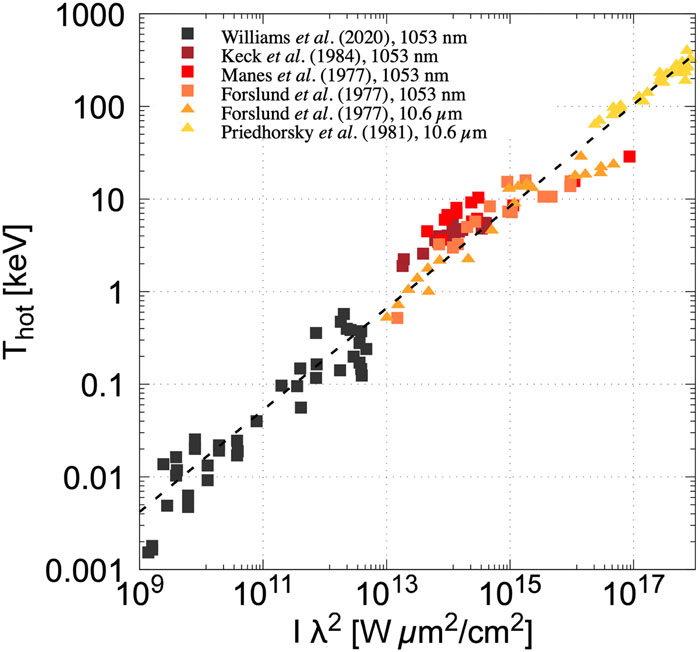
The source current I_d is expressed as $I_{d} (t) = e h \frac{I_{L} π r_{L}^{2}}{2 k_{B} T_{hot}} [1 + \frac{e V (t)}{k_{B} T_{hot}}] e^{- e V (t) / k_{B} T_{hot}},$ (3)where h is the conversion rate from the laser intensity to the hot-electron flux and r_L is the laser focal radius.22 A square pulse is often used for the incident laser of the laser-driven coil, and thus the laser intensity I_L and hot-electron temperature T_hot can be considered to be constant during the laser pulse. In the GEKKO-XII facility, a Gaussian pulse is used for the incident laser, and thus I_L and T_hot are time-dependent parameters. This time dependence should be considered in the circuit model.

We now give detailed descriptions of the calculation of the coil current I(t) and voltage V(t) using the self-consistent circuit model given by Eqs. (1)–(3). Based on a previous magnetic field measurement conducted at the GEKKO-XII facility with a Gaussian laser pulse,25 we set the total energy, pulse duration (FWHM), focal spot size (diameter), and wavelength of the incident laser to 540 J, 1.3 ns, 50 µm, and 1053 nm, respectively. The peak intensity of the Gaussian pulse was obtained using the relation 0.94I_Square = I_Gauss to make the total energy of the two types of laser pulse the same; the value of I_Gauss was calculated to be 1.99 × 10¹⁶ W/cm². The hot-electron temperature generated by laser irradiation was evaluated based on the laser intensity scaling using the following relation: $\begin{align} T_{hot} = 5.7 {(I_{L} λ_{L}^{2} [(\times 1 0^{15} {W / c m}^{2}) μ m^{2}])}^{0.55} [k e V] . \end{align}$ (4)This intensity scaling can be obtained from experimental results,26–30 as shown in Fig. 1. In Refs. 24 and 26, an appropriate intensity scaling that depended on laser intensity was used; by contrast, our analysis uses wide-range intensity scaling. To model the effects of pulse shape on the hot-electron temperature, we assume that the hot-electron temperature at some arbitrary time depends only on the laser intensity at that time, i.e., $T_{hot} (t) = T_{hot} (I_{L} (t))$ . This assumption is valid for a pulse longer than 100 ps, based on the experimental results shown in Fig. 1.

Figure 1.Laser intensity scaling of hot-electron temperature.^26–30 Squares (■) and triangles (▴) represent laser wavelengths of 1053 nm and 10.6 µm, respectively.

The self-consistent circuit model requires a numerical simulation to obtain the R(t) in Eq. (2). Thus, we ran a two-dimensional cylindrical simulation to calculate R(t), taking account of current diffusion and Joule heating.

Figure 2 shows the calculation geometry. The ring-shaped coil was modeled with a coil radius of 250 µm and a wire diameter of 50 µm in the calculation region. The voltage generated by the laser irradiation drives a current in the coil. To implement this voltage, we set up an azimuthal electric field parallel to the current direction. The generated voltage becomes an almost-Gaussian pulse when the incident laser uses a Gaussian pulse. Therefore, we imposed a Gaussian electric field in the first iteration of the numerical simulation. The imposed electric field is defined as E_ϕ,back(r, z, t) = E₀(t)r/a, where E₀(t) forms the Gaussian function and a represents the coil radius. The total electric field is expressed as E = E_back + E_ind, where E_ind is the electric field that results from the time-changing magnetic field. The background electric field generates a background magnetic field such that $B_{z, back} (t) = - \int_{0}^{t} d t^{'} {(\nabla \times E_{back} (t^{'}))}_{z} = - \int_{0}^{t} d t^{'} 2 E_{0} (t^{'}) / a$ . When the imposed electric field E₀(t) is given by a Gaussian function, the integral in B_z,back(t) can be calculated with the Gaussian error function as follows: $\int_{0}^{t} d t^{'} e^{- {(α t^{'})}^{2}} = \frac{1}{α} \int_{0}^{α t} d t^{'} e^{- t^{' 2}} = \frac{\sqrt{π}}{2 α} erf (α t) .$ (5)The total magnetic field is expressed as B = B_back + B_ind. Our focus is on the magnetic field generated by the current in the coil, B_ind, and therefore we subtracted the background magnetic field B_back from the calculated magnetic field B.

Figure 2.Calculation geometry and initial condition of the cylindrical simulation. The ring-shaped coil (nickel) was modeled with a coil radius of 250 µm and a wire diameter of 50 µm. The background field, E_ϕ,back, was initially imposed.

In this transient simulation, the electric and magnetic fields were calculated numerically from the following Maxwell’s equations: $\begin{align} \frac{\partial E_{ind}}{\partial t} = \frac{1}{μ ε} \nabla \times B_{ind} - \frac{σ}{ε} (E_{back} + E_{ind}) - \frac{\partial E_{back}}{\partial t}, \end{align}$ (6) $\begin{align} \frac{\partial B_{ind}}{\partial t} = - \nabla \times (E_{ind} + E_{back}) - \frac{\partial B_{back}}{\partial t} = - \nabla \times E_{ind}, \end{align}$ (7)where μ, ε, and σ are the permeability, permittivity, and electrical conductivity, respectively. The finite-difference time-domain method31 was applied to solve these equations in cylindrical coordinates. The azimuthal electric field E_ϕ was calculated using the following difference equation: $\begin{align} E_{ϕ, i n d}^{n} (i, j) = e^{- (σ / ε) Δ t} [E_{ϕ, b a c k}^{n - 1} (i, j) + E_{ϕ, i n d}^{n - 1} (i, j)] \\ + \frac{1 - e^{- (σ / ε) Δ t}}{σ} {[\frac{\partial H_{r, ind}}{\partial z} (i, j) - \frac{\partial H_{z, ind}}{\partial r} (i, j)]}^{n - \frac{1}{2}} . \end{align}$ (8)

The radial and axial magnetic fields H_r and H_z, respectively, were calculated as $\begin{align} H_{r, i n d}^{n + \frac{1}{2}} (i, j) = H_{r, i n d}^{n - \frac{1}{2}} (i, j) + {[\frac{Δ t}{μ} \frac{\partial E_{ϕ, i n d}^{n}}{\partial z} (i, j)]}^{n}, \end{align}$ (9) $\begin{align} H_{z, i n d}^{n + \frac{1}{2}} (i, j) = H_{z, i n d}^{n - \frac{1}{2}} (i, j) - \frac{1}{r} \frac{Δ t}{μ} \frac{\partial}{\partial r} [r E_{ϕ, i n d}^{n} (i, j)] . \end{align}$ (10)Simulations were run from 0.0 to 10.0 ns. The computational boundary and mesh size were set to 1000 × 2000 µm² and 2 µm, respectively. The time step was 6.67 fs with Courant’s restriction.

The coil was modeled in a two-dimensional simulation with cylindrical coordinates, and thus the resistance obtained was that for a ring-shaped coil. The actual coil was modeled in a static calculation.32 The ratio of the two- and three-dimensional coil resistances, R_3D/R_2D, was calculated to be 1.38. We used this scaling factor to convert the two-dimensional resistance and voltage to three-dimensional values in the iteration process. The simulation showed that the temporal evolution of the coil inductance is negligible, and thus we set the coil inductance to be 1.37 nH for the actual shape.32

Joule heating was implemented as c_Vρ∂T/∂t = σ(T)|E_ϕ + E_ϕ,back|², where c_V and ρ are the isochoric specific heat and density, respectively. Thermal diffusion is too small to matter on the experimental timescale and was therefore ignored in this simulation. The laser-driven coil often used in the GEKKO-XII and LULI (at École Polytechnique) facilities is made of nickel. The specific heat and mass density were set to 440 J/(kg K) and 7.81 g/cm³, respectively. We calculated the electrical conductivity of nickel at temperatures above 0.3 eV with the Lee–More–Desjarlais model.33,34 The application of this model instead of the quantum approach described later is reliable because nickel has a lower atomic number and density than those of gold. At temperatures below 0.3 eV, we used experimental data.35

Figure 3(a) shows the temporal evolution of the coil current and voltage, with the temperature dependence of the nickel conductivity taken into account. As the voltage increases, the coil current slowly increases, reaching its maximum at 4.2 ns. Because of the coil inductance, the coil current is delayed by 1.4 ns with respect to the voltage. Unlike the voltage evolution, the coil current differs from a Gaussian pulse, because the coil resistance changes dramatically until 4.2 ns. After the peak at 4.2 ns, the current starts to decay with L/R(t), which is longer than the turn-off time of the voltage.

Figure 3.Temporal evolution of (a) self-consistent voltage and current and (b) coil resistance. The coil current increases slowly, reaching a maximum at 4.2 ns. The coil resistance changes dramatically until 4.2 ns.

Figure 3(b) shows the temporal evolution of the coil resistance taking account of current diffusion and Joule heating. The coil resistance initially decreases owing to current diffusion (up to 800 ps). After 800 ps, the surface of the coil starts to heat up dramatically, and the total resistance increases (the conductivity decreases), reaching a maximum value of 3.1 Ω at 1.9 ns. This indicates that the coil temperature increases up to ∼4 eV until this time. Note that because the coil cross-section is small (the coil diameter is 50 µm), the current density diffuses over almost the entire cross-section in 2 ns. The conductivity of nickel increases above 4 eV, and thus the coil resistance decreases over time. The small temporal fluctuation of the coil resistance does not significantly affect the temporal evolution of the coil current.

III. ELECTRICAL CONDUCTIVITY OF WARM DENSE GOLD

The electrical conductivity of gold was calculated in the range of 300 K–100 eV. Figure 4 shows the electrical conductivity of warm dense gold at a density of 19.3 g/cm³ vs temperature. For T < 0.27 eV, experimental data were used. For 0.27 eV < T < 7 eV, the conductivity was calculated using the Kubo–Greenwood formula based on a quantum MD simulation. For T > 7 eV, the conductivity was calculated using the modified Spitzer formula. The details are described below.

Figure 4.Temperature dependence of the electrical conductivity of solid dense gold. For T < 0.27 eV, experimental data were used. For 0.27 eV < T < 7 eV, the conductivity was calculated using the Kubo–Greenwood formula based on a quantum MD simulation. For T > 7 eV, the conductivity was calculated with the modified Spitzer formula.

For the temperature range 0.27 eV < T < 7 eV, we estimated the electrical conductivity of warm dense gold with a quantum MD simulation in conjunction with the Kubo–Greenwood formula. The quantum MD simulation was performed to calculate the temporal evolution of ionic configurations using the Vienna Ab initio Simulation Package (VASP)36 based on the Nosé–Hoover thermostat.37

The electron orbitals and the eigenenergies for the transport properties were calculated using plane-wave Kohn–Sham density functional theory with the ABINIT code.38 The quantum MD calculations were performed in the period 2–4 ps with a time step of 2 fs. Thirty-two atoms were treated in a supercell. For each atom, 11 electrons (5d¹⁰6s¹) under the projected augmented wave pseudopotential39 were taken into account in the calculation. The cutoff energy was set to 600 eV. The single special point representing multiple k-points was used for MD steps to reduce the computational cost. The special point concept was proposed to reduce the k-points sampling based on crystal symmetry.40,41 This method is also empirically applicable to types of liquid-like structure such as WDM. The generalized gradient approximation using the Perdew–Burke–Ernzerhof functional was used as the exchange-correlation potential.42 In the ground state calculation, 2³k-points were sampled in the Brillouin zone with the Monkhorst–Pack scheme.40,41

The electrical conductivity at a given frequency ω can be calculated using the Kubo–Greenwood formula $\begin{align} σ (ω) = \frac{2 π e^{2} ℏ^{2}}{3 m_{e}^{2} Ω ω} \sum_{n, m, k} [f (ɛ_{m}^{k}) - f (ɛ_{n}^{k})] \\ \times {|〈 ψ_{n}^{k} | \nabla | ψ_{m}^{k} 〉|}^{2} δ (ɛ_{n}^{k} - ɛ_{m}^{k} - ℏ ω) . \end{align}$ (11)Here m_e, ℏ, and Ω are the electron mass, Dirac constant, and volume of a supercell, respectively. $f (ɛ_{n}^{k})$ is the Fermi distribution function and describes the occupation of the n-th band corresponding to the energy $ɛ_{n}^{k}$ and the wave function $ψ_{n}^{k}$ at the k-point k.

To obtain the DC electrical conductivity, we extrapolated the DC limit with the Drude conductivity curve, which represents the free-electron contribution $σ (ω) = \frac{σ_{0}}{1 + ω^{2} τ^{2}},$ (12)where σ₀ and τ are the DC conductivity and collisional relaxation time of free electrons, respectively. In this calculation, the delta function in Eq. (11) is replaced with the following Gaussian: $\frac{1}{\sqrt{π} Δ} e^{- {(x / Δ)}^{2}} .$ (13)The parameter Δ was set to 1.36 eV (0.05 hartree). The values were averaged for five snapshots of an MD trajectory to reduce statistical error.

We confirmed that the DC limit of the optical properties converges numerically with 3³ and 4³k-points sampling. The numerical fluctuation of the optical conductivity at low frequency can be reduced by using a large number of k-points. The statistical error with 2³k-points sampling was reduced by taking the average of five snapshots. We also confirmed that the DC limit of the optical properties numerically converges with 54 and 108 atoms. The convergence of the DC limit sometimes requires a vast number of atoms (e.g., 1000) to increase the size of the supercell at a given density.43 We used only 32 atoms in the calculation because computations with such large numbers of atoms are impractical for a high-Z material such as gold. The DC conductivity obtained with 32 atoms is similar to that obtained with 54 atoms. Our results also agree with the conductivity obtained with 108 atoms.44

The projected augmented wave method, which assumes cold core electrons for a single atom, does not provide exact results at high temperatures. We thus evaluated the electrical conductivity using the quantum MD simulation for warm dense conditions below 7 eV system temperature. For temperatures above 7 eV, the electrical conductivity was calculated using the modified Spitzer–Härm formula20 given by $σ (T) = γ (Z_{ion}) \frac{T^{\frac{3}{2}}}{38 Z_{ion} \ln Λ},$ (14)where ln Λ, γ, and Z_ion are the Coulomb logarithm, electron correlation factor, and ion charge state, respectively. The Coulomb logarithm proposed by Zaghloul et al.45,46 was used in this calculation. The electron correlation factor47 describes the effect of electron degeneracy, and is given by a fitting function as follows: $γ (Z_{ion}) = \frac{3 π}{32} (1 + \frac{153 Z_{ion}^{2} + 509 Z_{ion}}{64 Z_{ion}^{2} + 345 Z_{ion} + 288}) .$ (15)The ionization state was calculated using the nonideal Saha equation, which contains continuum lowering due to the electron screening effect $\frac{n_{z} n_{e}}{n_{z - 1}} = 2 \frac{U_{z}}{U_{z - 1}} {(\frac{m_{e} k_{B} T}{2 π ℏ^{2}})}^{\frac{3}{2}} \exp (- \frac{I_{z}^{eff}}{k_{B} T}),$ (16)where n_z and U_z are the number density and internal portion function for z-fold ions. $I_{z}^{eff}$ is the effective ionization energy, i.e., I_z − ΔI_z, from z − 1 to z. The correction to the ionization energy, ΔI_z (potential lowering), was calculated as follows: $Δ I_{z} = \frac{(z + 1) e^{2}}{\sqrt{λ_{D}^{2} + {(\frac{2}{3} a_{z})}^{2}}},$ (17)where λ_D and a_z are the Debye length and ion sphere radius for z-fold ions, respectively. The excited state data, such as U_z and I_z in Eq. (16), were taken from a database compiled by the National Institute of Standards and Technology.48

At low temperatures (≲0.2 eV), where the atoms are ordered periodically, material conductivity is primarily determined by electron–phonon scattering (especially Umklapp scattering), which changes the momentum. The Kubo–Greenwood expression does not account for this mechanism, and the DC limit of the Kubo–Greenwood expression is no longer valid.49,50 Thus, the conductivity at a temperature below the boiling point T_b = 0.27 eV was obtained from the empirical fitting formula αT⁻ⁿ based on experimental results,51 where α and n are fitting parameters. For the solid phase, i.e., at temperatures below the melting temperature T_m = 0.12 eV, we find that α = 6.90 × 10⁵ and n = 1.14 provide the best fit to the experimental data. For the liquid phase, at temperatures below the boiling temperature T_b = 0.27 eV, we find that α = 7.91 × 10⁵ and n = 0.65 provide the best fit.

IV. MAGNETIC DIFFUSION INTO GOLD CONE TARGET

We also performed two-dimensional simulations to investigate how the magnetic field generated by the laser-driven coil discussed in Sec. II diffuses into the guiding cone, which has the σ(T) calculated in Sec. III. In this simulation, we used the obtained coil current shown in Fig. 3 as a current source to analyze the magnetic diffusion under the assumption that the current density distribution in the coil is uniform during the simulation and the mutual induction on the source current is negligibly small. The current density distribution only slightly affects the magnetic field distribution, because the cross-section of the modeled laser-driven coil is sufficiently small compared with the coil radius.

The azimuthal electric field E_ϕ was calculated using the following difference equation: $\begin{align} E_{ϕ}^{n} (i, j) = - \frac{1 - e^{- (σ / ε) Δ t}}{σ} j_{ϕ}^{n - 1} (i, j) \\ + e^{- (σ / ε) Δ t} E_{ϕ}^{n - 1} (i, j) \\ + \frac{1 - e^{- (σ / ε) Δ t}}{σ} {[\frac{\partial H_{r}}{\partial z} (i, j) - \frac{\partial H_{z}}{\partial r} (i, j)]}^{n - \frac{1}{2}} . \end{align}$ (18)

The magnetic field was solved using the difference Eqs. (9) and (10) (see Sec. II).

The target configuration (laser-driven coil and guiding cone) in this simulation was set to be the same as that in a previous MFI integrated experiment.15,16 The specific heat and mass density of the solid gold were 129 J/(K kg) and 19.3 g/cm³. The simulation conditions were set to be the same as those in the transient simulation discussed in Sec. III.

Figure 5 shows the temporal evolution of the incident laser pulse (dashed line), the magnetic field generated in vacuum (solid blue line), and the magnetic field that penetrated the gold cone with a previously reported σ(T)19 (solid green line) and the σ(T) shown in Fig. 4 (solid red line).

Figure 5.Temporal evolution of the incident laser pulse (dashed black line), the magnetic field generated in vacuum (solid blue line), and the magnetic field that penetrated the gold cone with a previously reported σ(T)¹⁹ (solid green line) and the σ(T) shown in Fig. 4 (solid red line), respectively. The square point shows the experimental data on the magnetic field measured inside a plastic insulator (corresponding to vacuum).²⁵ The shaded area (4.8–5.2 ns) represents the time window in the arrival times of several shots of a short-pulse laser to heat the fuel core in the previous MFI experiment.¹⁵

A single data point is provided from Ref. 25, which was measured inside a plastic insulator using proton deflectometry. Two laser-driven coils were used in a Helmholtz geometry in this experiment, although the coil-centered field is not expected to deviate significantly from the field of a single laser-driven coil. A plastic insulator was placed at the middle of the Helmholtz geometry so that the laser-produced plasma did not affect the proton-deflectometry measurements. Comparison with proton ray-tracing simulations suggests that the magnetic field diffused quickly into the plastic and that the measurements were equivalent to those in a vacuum.

The incident laser is a Gaussian pulse whose FWHM is 1.3 ns and whose peak is at 3 ns. In a vacuum, the magnetic field at the center of the coil has the same temporal evolution as that of the coil current. The generated magnetic field increases over time, reaching a maximum strength of 600 T at 4.2 ns. The time delay from the peak of the incident laser intensity to the peak of the generated magnetic field was calculated to be 1.2 ns. This delay is approximately consistent with the results of a magnetohydrodynamic simulation.52 The magnetic fields inside the gold cone when using previous and recent σ(T) are almost zero until 2.0 ns, because the cone retains high conductivity. Once the gold cone heats up to the melting temperature (0.12 eV), the magnetic field begins to diffuse into the gold cone and gradually increases. Consequently, the magnetic field that penetrates the gold cone reaches a maximum strength of 560 T at 4.9 ns and 530 T at 5.5 ns using previous and recent σ(T), respectively, The maximum magnetic field that penetrates the cone is delayed by 2.5 ns with respect to the laser peak for our recent simulation.

In the MFI experiments performed by Sakata et al.15 and Matsuo et al.,16 a heating laser with 1.5-ps duration arrived 1.88–2.22 ns after the peak of the coil drive laser (the shaded area in Fig. 5). The maximum coupling efficiency was observed 2.2 ns after the incident laser. To help explain this observation, we discuss distributions of the wall temperature on the guiding cone and the magnetic field at 5.2 ns (i.e., 2.2 ns after the laser peak at 3 ns).

Figure 6(a) shows the two-dimensional profile of the cone temperature 2.2 ns after the peak of the incident laser pulse (i.e., at 5.2 ns in the simulation). The cone wall heats up to several tens of electron volts owing to the induction heating caused by the applied magnetic field. In this temperature range, the electrical conductivity of gold is an order of magnitude lower than that at room temperature, leading to rapid magnetic diffusion. Figure 6(b) shows the two-dimensional profile of the simulated magnetic field 2.2 ns after the peak of the incident laser pulse. The generated magnetic field penetrates the 7-μm-thick cone wall sufficiently at this time, as also shown in Fig. 5.

Figure 6.Spatial distributions of (a) temperature and (b) magnetic field at 5.2 ns. The cone wall heats up to several tens of electron volts owing to induction heating, and the electrical conductivity drops by an order of magnitude. This conductivity drop leads to rapid diffusion, and thus the applied magnetic field penetrates the cone wall at this time.

The magnetic field strength at the cone tip is important for guiding the REB by an external magnetic field. Our numerical analysis reveals that the applied magnetic field penetrates the guiding cone sufficiently and that the magnetic field has sufficient strength at the cone tip to guide the REB to the fuel core at a time when the heating laser was incident in previous MFI experiments.15,16

Figure 7 shows the line-outs of the simulated magnetic field strength at 5.2 ns [Fig. 6(b)] on the z axis obtained with (i) a constant electrical conductivity of 4.07 × 10⁷ S/m, which is the value at room temperature, (ii) the temperature-dependent electrical conductivity based on a previous analysis,19 and (iii) the temperature-dependent electrical conductivity shown in Fig. 4. For the simulation with constant conductivity, the magnetic field strength at the coil center (z = 225 µm) is 15.6 T, which means that the magnetic field cannot penetrate the cone wall until 5.2 ns. For the simulations with time-varying conductivities, the magnetic field strengths are 560 and 530 T for (ii) and (iii), respectively, as shown in Fig. 5. At the cone tip (z = 100 µm), the magnetic field strength for (i) is 102 T, which is relatively weak, and those for (ii) and (iii) are 397 and 385 T, respectively. Although the magnetic field strength for (iii) is slightly weaker than that for (ii), it is still sufficiently strong to guide the REB to the fuel core, as discussed in a previous study.14,19

Figure 7.Line-outs of the magnetic field strength at 5.2 ns on the z axis with (i) a constant electrical conductivity of 4.07 × 10⁷ S/m, (ii) the temperature-dependent electrical conductivity based on a previous analysis,¹⁹ and (iii) the temperature-dependent electrical conductivity shown in Fig. 4. The magnetic field strengths at the cone tip are 102, 385, and 397 T, respectively.

V. SUMMARY

In summary, we have developed a model of magnetic field generation valid for laser-driven coils with thin wire loops, and we have improved a previous analysis of magnetic field diffusion into the gold guiding cone.

For the generation process, we calculated the temporal evolution of the coil current and laser-generated magnetic field in the laser-driven coil using the self-consistent circuit model. The peak of the calculated magnetic field is delayed by 1.2 ns compared with that of the incident laser pulse. For the diffusion process, we calculated the electrical conductivity of warm dense gold over a wide temperature range (300 K–100 eV) using a combination of the Kubo–Greenwood formula based on a quantum MD simulation and the modified Spitzer model to estimate the magnetic diffusion into the guiding cone target, taking account of the temperature dependence of the electrical conductivity. The magnetic field that penetrates the gold cone reaches a maximum strength of 530 T at 5.5 ns. The maximum magnetic field that penetrates the cone is delayed by 2.5 ns with respect to the laser peak. In the MFI experiments performed by Sakata et al.15 and Matsuo et al.,16 a heating laser was irradiated 1.88–2.22 ns after the incident laser peak of the laser-driven coil. The maximum coupling efficiency was observed 2.2 ns after the incident laser. At this timing, the calculation shows that the field strength at the tip of the gold cone is 385 T, which is sufficiently strong to guide the REB to the fuel core.

In magnetized high-energy-density plasma experiments with intense magnetic pulses, the temperature of sample materials increases dramatically owing to induction heating accompanied by magnetic diffusion, and the electrical and thermal conductivities both change over time. Knowledge of the temperature dependence of transport properties such as the electrical conductivity over a wide temperature range is essential for numerically evaluating intense field dynamics. Our results contribute to the modeling of a high-power laser-driven coil and the estimation of intense magnetic diffusion.

ACKNOWLEDGMENTS

Acknowledgment. The authors wish to thank the technical support staff of the Institute of Laser Engineering at Osaka University and the High Energy Density Science Center at the Lawrence Livermore National Laboratory for hosting H. Morita on the Quartz Supercomputer, where portions of this research were done. The authors appreciate greatly valuable discussions with Dr. S. X. Hu and V. V. Karasiev (Univ. Rochester, Laboratory for Laser Energetics). This work was supported by a Grant-in-Aid for JSPS Research Fellow (Grant No. 20J10496), KAKENHI (Grant Nos. 15KK0163, 16K13918, and 16H02245), the Osaka University Scholarship for Overseas Research Activities 2018, Japan/U.S. Cooperation in Fusion Research and Development, the Matsuo Research Foundation, and the Research Foundation for Opto-Science and Technology. Part of this work was performed under the auspices of the U.S. Department of Energy by Lawrence Livermore National Laboratory under Contract No. DE-AC5207NA27344.

APPENDIX: SIMPLE ANALYSIS OF INDUCTION HEATING THROUGH MAGNETIC DIFFUSION

An intense magnetic pulse such as that created by a laser-generated magnetic field causes induction heating in a conductor. We need to carefully consider the temperature dependence of the electrical conductivity to estimate the magnetic diffusion time. Here, we estimate the temperature increase in a metal as a result of induction heating when a magnetic pulse is applied.

Assume that a parallel magnetic field in the x direction is applied to only the outside (z < 0) of the conductor, whose thickness is d, as shown in Fig. 8. The high-frequency modes of this pulsed magnetic field contribute to induction heating. We just consider a mode of B_x [A/(m s)], expressed as $B_{x} (z; ω) = b (z) e^{- i ω t} = B (ω) e^{- z / δ (ω)} e^{- i ω t},$ (A1)where δ(ω) is a skin depth for an oscillating field at a given frequency ω and is defined as (2/μσω)^1/2. To estimate the temperature increase, we can take the time average of this mode as follows: ${\bar{B}}_{x} (z; ω) = \frac{1}{\sqrt{2}} B (ω) e^{- z / δ (ω)} .$ (A2)When the magnetic pulse is a Gaussian pulse with FWHM of τ, a mode of the magnetic pulse, B(ω) [A/(m s)], is expressed as $\begin{align} B (ω) = B_{0} τ {(\frac{π}{4 \ln 2})}^{\frac{1}{2}} \exp [- \frac{{(ω τ)}^{2}}{16 \ln 2}] \\ = B_{0} \sqrt{4 π A} e^{- A ω^{2}}, \end{align}$ (A3)where A = τ²/(16 ln 2) and B₀ corresponds to the peak value of the magnetic pulse. Inside a conductor (z < 0), a mode of the current density, j_y(ω) [A/(m² s)], is obtained from Ampère’s law $\frac{1}{μ} \frac{\bar{B} (ω)}{δ (ω)} e^{- z / δ (ω)},$ (A4)A mode of the electric field, E_y(ω) [V/(m s)], can be obtained from Ohm’s law $\frac{1}{2} ω δ (ω) \bar{B} (ω) e^{- z / δ (ω)} .$ (A5)With Eqs. (A4) and (A5), the current density j_y [A/m] and the electric field E_y [V/m] inside the conductor are expressed as follows: $\begin{align} j_{y} = \frac{1}{μ} B_{0} \sqrt{4 π A} \sqrt{\frac{μ σ}{2}} \int_{0}^{\infty} d ω \sqrt{ω} e^{- α \sqrt{ω}} e^{- A ω^{2}}, \end{align}$ (A6) $\begin{align} E_{y} = \frac{1}{2} B_{0} \sqrt{4 π A} \sqrt{\frac{2}{μ σ}} \int_{0}^{\infty} d ω \sqrt{ω} e^{- α \sqrt{ω}} e^{- A ω^{2}} . \end{align}$ (A7)Here, we have replaced depth z with thickness d, and defined τ_dif ≡ μσd²/2 and $α = \sqrt{τ_{dif}}$ . From these equations, the induction heating j · E [W/m³], accompanied by magnetic diffusion can be expressed as $4 π A \frac{B_{0}^{2}}{2 μ} {(\int_{0}^{\infty} d ω \sqrt{ω} e^{- α \sqrt{ω}} e^{- A ω^{2}})}^{2} .$ (A8)The integral in parentheses cannot be calculated analytically, and so we expand $e^{- α \sqrt{ω}}$ as a series $e^{- α \sqrt{ω}} \sim \sum_{n} \frac{{(- α)}^{n}}{n!} ω^{n / 2} .$ (A9)The integral can then be written as $\sum_{n} \frac{{(- α)}^{n}}{n!} \int_{0}^{\infty} d ω ω^{(n + 1) / 2} e^{- A ω^{2}} .$ (A10)To deal with this integral, we can apply the following formula: $\int_{0}^{\infty} d x x^{2 k + 1} e^{- a x^{2}} = \frac{Γ (k + 1)}{2 a^{k + 1}},$ (A11)where Γ(x) is the gamma function. After substituting k = (n − 1)/4 into Eq. (A11), the expression (A8) can be written as $\begin{align} 4 π A \frac{B_{0}^{2}}{2 μ} {[\sum_{n} \frac{{(- α)}^{n}}{n!} \frac{Γ ((n + 3) / 4)}{2 A^{(n + 3) / 4}}]}^{2} \\ = \frac{4 π}{τ} \frac{B_{0}^{2}}{2 μ} {[\sum_{n} \frac{{(- 1)}^{n}}{n!} Γ (\frac{n + 3}{4}) {(\ln 2)}^{(n + 1) / 4} {(\frac{τ_{d i f}}{τ})}^{n / 2}]}^{2} . \end{align}$ (A12)Neglecting the thermal diffusion effect, we can obtain the temperature increase as follows: $\begin{align} Δ T = \frac{4 π}{c_{V} ρ} \frac{B_{0}^{2}}{2 μ} {[\sum_{n} \frac{{(- 1)}^{n}}{n!} Γ (\frac{n + 3}{4}) {(\ln 2)}^{(n + 1) / 4} {(\frac{τ_{dif}}{τ})}^{n / 2}]}^{2} \\ = \frac{1}{c_{V} ρ} \frac{B_{0}^{2}}{2 μ} {[\sum_{n} C_{n} {(\frac{τ_{dif}}{τ})}^{n / 2}]}^{2} . \end{align}$ (A13)The high-order series expansion of C_n in (A13) gives an accurate value. Here, we introduce the following fitting function of the high-order expansion: ${[\sum_{n} C_{n} {(\frac{τ_{dif}}{τ})}^{n / 2}]}^{2} \approx 5 π \frac{e^{- {(τ_{dif} / τ)}^{0.36}}}{1 + 0.51 τ_{dif} / τ} .$ (A14)We finally get the approximate temperature increase as $Δ T \approx \frac{1}{c_{V} ρ} \frac{B_{0}^{2}}{2 μ} \frac{5 π e^{- {(τ_{dif} / τ)}^{0.36}}}{1 + 0.51 τ_{dif} / τ} .$ (A15)The temperature increase ΔT expressed as in Eq. (A13) or Eq. (A15) depends on the ratio between diffusion time and pulse width, τ_dif/τ. The function (A14) is a monotonically decreasing function of τ_dif/τ. A long pulse (small τ_dif/τ) can heat the conductor for a long time, causing a large temperature increase. When the diffusion time is long (τ_dif/τ is large), the applied magnetic field does not soak into the conductor and thus does not significantly heat its inner surface. The expression (A14) converges to zero for large values of τ_dif/τ. This means that the applied magnetic field cannot penetrate the wall (thickness d) during the pulse duration; it heats only the surface of the conductor. Consequently, the inner surface is not heated (i.e., its temperature does not increase).

Figure 8.Simple illustration of magnetic diffusion. An infinitely wide conductive plate of thickness d is placed on the x–y plane. A magnetic field is applied in the x direction outside the conductor (0 < z). This magnetic field causes an eddy current in the y direction and diffuses into the conductive plate, causing induction heating.

Finally, we estimate the temperature increase of a gold foil as an example. The specific heat and density of solid gold are 129 J/(K kg) and 19.3 g/cm³. When a 1-ns Gaussian magnetic pulse of 600 T soaks into 10-μm-thick gold, the temperature increase can be calculated to be 1.59 eV (1.85 × 10⁴ K) using Eq. (A15). If the electrical conductivity drops by an order of magnitude owing to this temperature increase, the diffusion time will also drop by an order of magnitude. The estimated temperature increase is 20.7 eV (2.40 × 10⁴ K).

References

[1] W.Fox, S. X.Hu, D. H.Barnak, K.Germaschewski, D. B.Schaeffer, A.Bhattacharjee, D.Haberberger, G.Fiksel, R. K.Follett. High-Mach number, laser-driven magnetized collisionless shocks. Phys. Plasmas, 24, 122702(2017).

[2] H.Chen, A. E.Raymond, E.Del Rio, C.Mileham, J.Nees, P. T.Campbell, N.Alexander, L.Willingale, C.Stoeckl, A. G.Thomas, K.Krushelnick, M. S.Wei, A.Maksimchuk, W.Fox, P. M.Nilson, V.Chvykov, A.McKelvey, P.Fitzsimmons, V.Yanovsky, C.Zulick, A.Bhattacharjee, B.Hou, C. F.Dong. Relativistic-electron-driven magnetic reconnection in the laboratory. Phys. Rev. E, 98, 043207(2018).

[3] B. G.Logan, C. J.Werner, G. B.Zimmerman, L. J.Perkins. Two-dimensional simulations of thermonuclear burn in ignition-scale inertial confinement fusion targets under compressed axial magnetic fields. Phys. Plasmas, 20, 072708(2013).

[4] D.Nakamura, H.Sawabe, S.Takeyama, A.Ikeda, Y. H.Matsuda. Record indoor magnetic field of 1200 T generated by electromagnetic flux-compression. Rev. Sci. Instrum., 89, 095106(2018).

[5] J. P.Knauer, P. Y.Chang, R. D.Petrasso, R.Betti, C. K.Li, O. V.Gotchev, J. A.Frenje, M. J.-E.Manuel, J. R.Rygg, O.Polomarov, F. H.Séguin, D. D.Meyerhofer. Compressing magnetic fields with high-energy lasers. Phys. Plasmas, 17, 056318(2010).

[6] A.Sunahara, T.Johzaki, S.Fujioka, T.Watanabe, H.Nakashima, Z.Zhang, Y.Hironaka, N.Yamamoto, H.Nishimura, K.Shigemori, H.Shiraga, H.Azechi, K.Ishihara. Kilotesla magnetic field due to a capacitor-coil target driven by high power laser. Sci. Rep., 3, 1170(2013).

[7] C.Wang, G.Zhao, B.Zhu, D.Yuan, G.Liang, Y.Li, B.Han, J.Zhang, J.Zhu, N.Hua, F.Wang, H.Wei, Z.Zhang, B.Zhu, J.Zhong, Z.Fang, W.Jiang. Generation of strong magnetic fields with a laser-driven coil. High Power Laser Sci. Eng., 6, e38(2018).

[8] G.Zhao, S.Kondo, H. G.Wei, K.Zhang, Y.Hara, X. X.Pei, Y.Sakawa, Y. T.Li, Z.Zhang, Y. F.Li, G. Y.Liang, B. J.Zhu, S.Fujioka, F. L.Wang, J. Y.Zhong, T.Sano. Magnetic reconnection driven by Gekko XII lasers with a Helmholtz capacitor-coil target. Phys. Plasmas, 23, 032125(2016).

[9] K.Matsuo, Y.Sakawa, S.Sakata, Z.Zhang, S.Kojima, P.Nicolai, Y.Arikawa, H.Azechi, H.Nagatomo, Y.Kuramitsu, T.Sano, T.Morita, S. H.Lee, S.Fujioka, K. F. F.Law. Magnetohydrodynamics of laser-produced high-energy-density plasma in a strong external magnetic field. Phys. Rev. E, 95, 053204(2017).

[10] T.Morita. Topological investigation of laser ion acceleration. Plasma Phys. Controlled Fusion, 62, 105003(2020).

[11] T.Yabuuchi, K. U.Akli, J. S.Green, D. S.Hey, C. D.Murphy, R.Kodama, R. J.Clarke, P.Simpson, C.Stoeckl, R.Stephens, J. R.Davies, P. A.Norreys, K. L.Lancaster, H.Habara, M.Zepf, R. R.Freeman, K.Krushelnick, M.Nakatsutsumi, M. H.Key. Measurements of energy transport patterns in solid density laser plasma interactions at intensities of 5 ×10²⁰ W cm⁻². Phys. Rev. Lett., 98, 125002(2007).

[12] R. G.Evans, J. A.King, K. U.Akli, V. M.Ovchinnikov, M.Zepf, F. N.Beg, Z.Najmudin, H.Azechi, H.Habara, C.Bellei, J.Waugh, K. A.Tanaka, R.Stephens, A.McPhee, R. R.Freeman, K. L.Lancaster, L.Van Woerkom, R.Heathcote, T.Tanimoto, N. C.Lopes, M. H.Key, J. R.Davies, K.Takeda, T.Ma, K.Markey, N. C.Woolsey, R.Onofrei, P. A.Norreys, J. S.Green, P.Nilson, W.Theobald, A. J.MacKinnon. Effect of laser intensity on fast-electron-beam divergence in solid-density plasmas. Phys. Rev. Lett., 100, 015003-015004(2008).

[13] H.-b.Cai, S.-p.Zhu, X. T.He. Effects of the imposed magnetic field on the production and transport of relativistic electron beams. Phys. Plasmas, 20, 072701(2013).

[14] J.-R.Marquès, R.Bouillaud, J. E.Cross, J.-L.Dubois, G.Gregori, D.Batani, N.Woolsey, J. J.Santos, Z.Zhang, L.Giuffrida, V. T.Tikhonchuk, R.Crowston, S.Dorard, S.Kojima, M.Bailly-Grandvaux, E.Loyez, S.Hulin, S.Sakata, J.Servel, A.Morace, P.Forestier-Colleoni, J. J.Honrubia, M.Ehret, M.Chevrot, P.Nicola?, F.Serres, C.Bellei, G.Schaumann, M.Roth, S.Fujioka. Guiding of relativistic electron beams in dense matter by laser-driven magnetostatic fields. Nat. Commun., 9, 102(2018).

[15] S.Sakata, T.Norimatsu, S.Kojima, Y.Arikawa, Y.Sentoku, K.Mima, T.Shiroto, H.Sakagami, A.Syuhada, N.Miyanaga, H.Morita, M.Nakai, A.Morace, T.Ozaki, R.Kodama, A.Yao, N.Iwata, H.Sawada, Y.Abe, H.Kishimoto, K. F. F.Law, Y.Nakata, S.Lee, H.Nishimura, T.Johzaki, K.Matsuo, J.Kawanaka, J. J.Santos, A.Yogo, K.Yamanoi, A.Sunahara, S.Fujioka, H.Azechi, H.Shiraga, Y.Iwasa, M.Hata, S.Tokita, M.Bailly-Grandvaux, H.Nagatomo. Magnetized fast isochoric laser heating for efficient creation of ultra-high-energy-density states. Nat. Commun., 9, 3937(2018).

[16] A.Sunahara, K. F. F.Law, T.Sano, M.Hata, Y.Iwasa, A.Yogo, H.Azechi, S.Kojima, H.Sakagami, Y.Abe, S.Lee, H.Nagatomo, S.Fujioka, N.Higashi, M.Nakai, H.Morita, H.Shiraga, S.Tokita, N.Iwata, Y.Arikawa, H.Sawada, Y.Ochiai, K.Matsuo, T.Norimatsu, Y.Nakata, A.Morace, K.Mima, S.Sakata, K.Yamanoi, T.Johzaki, R.Kodama, T.Ozaki, Y.Sentoku, J.Kawanaka. Petapascal pressure driven by fast isochoric heating with a multipicosecond intense laser pulse. Phys. Rev. Lett., 124, 035001(2020).

[17] K. S.Anderson, G.Fiksel, W.Theobald, C.Stoeckl, A. A.Solodov, R. B.Stephens, L. C.Jarrott, T. C.Sangster, G.McKiernan, J. J.Santos, H. S.McLean, H.Sawada, F. N.Beg, A.Shvydky, R.Epstein, V. Y.Glebov, F. J.Marshall, M. S.Wei, P. K.Patel, S.Ivancic, E. M.Giraldez, F.Pérez, P. M.Nilson, C.Mileham, H.Habara. Time-resolved compression of a capsule with a cone to high density for fast-ignition laser fusion. Nat. Commun., 5, 5785(2014).

[18] F. N.Beg, B.Qiao, H. S.Mclean, P. K.Patel, C.Stoeckl, M. S.Wei, C.McGuffey, J. J.Santos, E. M.Giraldez, W.Theobald, H.Chen, R. B.Stephens, R. W.Luo, T.D?ppner, T.Yabuuchi, J.Delettrez, T.Iwawaki, V. Y.Glebov, C.Mileham, A. A.Solodov, L. C.Jarrott, R.Betti, H.Habara, M. H.Key, F. J.Marshall, H.Sawada. Visualizing fast electron energy transport into laser-compressed high-density fast-ignition targets. Nat. Phys., 12, 499-504(2016).

[19] H.Azechi, A.Sunahara, S.Fujioka, H.Morita, Y.Arikawa. Numerical analysis of pulsed magnetic field diffusion dynamics in gold cone target. Phys. Plasmas, 25, 094505(2018).

[20] X.Sun, L.Jia, Z.Fu, Q.Chen. Electrical conductivity of warm dense tungsten. High Energy Density Phys., 9, 781-786(2013).

[21] C. S.Goyon, K. F. F.Law, H.Morita, S.Fujioka, G. J.Williams, J. D.Moody, B. B.Pollock. Dynamics of laser-generated magnetic fields using long laser pulses. Phys. Rev. E, 103, 033201(2021).

[22] D. M.Chambers, C.Courtois, N. C.Woolsey, R. A. D.Grundy, A. D.Ash. Creation of a uniform high magnetic-field strength environment for laser-driven experiments. J. Appl. Phys., 98, 054913(2005).

[23] W.Fox, L.Gao, G.Fiksel, H.Ji. A simple model for estimating a magnetic field in laser-driven coils. Appl. Phys. Lett., 109, 134103(2016).

[24] J. J.Santos, A.Poyé, M.Bailly-Grandvaux, V. T.Tikhonchuk. Quasi-stationary magnetic field generation with a laser-driven capacitor-coil assembly. Phys. Rev. E, 96, 023202(2017).

[25] K. F. F.Law, Z.Zhang, S.Sakata, H.Azechi, S.Kojima, M.Bailly-Grandvaux, K.Kondo, S.Fujioka, C.Bellei, A.Morace, A.Yogo, S.Lee, Y.Arikawa, X.Vaisseau, K.Matsuo, J. J.Santos. Direct measurement of kilo-tesla level magnetic field generated with laser-driven capacitor-coil target by proton deflectometry. Appl. Phys. Lett., 108, 091104(2016).

[26] S.Patankar, J. D.Bude, V. T.Tikhonchuk, G. J.Williams, B. B.Pollock, J. D.Moody, C.Goyon, M. A.Norton, D. A.Mariscal, E. R.Tubman, C. W.Carr, G. F.Swadling, A. M.Rubenchik. Laser intensity scaling of the magnetic field from a laser-driven coil target. J. Appl. Phys., 127, 083302(2020).

[27] L. M.Goldman, R. L.Keck, K.Tanaka, M. C.Richardson, W.Seka. Observations of high-energy electron distributions in laser plasmas. Phys. Fluids, 27, 2762(1984).

[28] R. A.Haas, H. G.Ahlstrom, J. F.Holzrichter, K. R.Manes. Light-plasma interaction studies with high-power glass laser. J. Opt. Soc. Am., 67, 717-726(1977).

[29] K.Lee, D. W.Forslund, J. M.Kindel. Theory of hot-electron spectra at high laser intensity. Phys. Rev. Lett., 39, 284-287(1977).

[30] W.Priedhorsky, D.Lier, D.Gerke, R.Day. Hard-x-ray measurements of 10.6-μm laser-irradiated targets. Phys. Rev. Lett., 47, 1661-1664(1981).

[31] S.Christian, F.Wolfgang, C.Andreas. Review of FDTD time-stepping schemes for efficient simulation of electric conductive media. Microwave Opt. Technol. Lett., 25, 16-21(2000).

[32] S.Fujioka, G.Korn, D.Margarone, L.Giuffrida, M.De Marco, F.Schillaci, Z.Zhang. Numerical simulations to model laser-driven coil-capacitor targets for generation of kilo-Tesla magnetic fields. AIP Adv., 8, 025103(2018).

[33] R. M.More, Y. T.Lee. An electron conductivity model for dense plasmas. Phys. Fluids, 27, 1273(1984).

[34] M. P.Desjarlais. Practical improvements to the Lee-More conductivity near the metal-insulator transition. Contrib. Plasma Phys., 41, 267(2001).

[35] M.Yousuf, P. C.Sahu, G. K.Rajan. High-pressure and high-temperature electrical resistivity of ferromagnetic transition metals: Nickel and iron. Phys. Rev. B, 34, 8086(1986).

[36] G.Kresse, J.Furthmüller. Efficient iterative schemes for ab initio total-energy calculations using a plane-wave basis set. Phys. Rev. B, 54, 11169(1996).

[37] S.Nosé. A unified formulation of the constant temperature molecular dynamics methods. J. Chem. Phys., 81, 511-519(1984).

[38] M.Stankovski, M. J.Verstraete, M.Delaveau, D.Caliste, D. R.Hamann, F.Da Pieve, D.Adams, C.Espejo, T.Rangel, I.Luka?evi?, Y.Pouillon, Y.Gillet, A.Levitt, A.Bokhanchuk, F.Jollet, M. J. T.Oliveira, E.Bousquet, S.Poncé, X.Gonze, G.Geneste, O.Rubel, A.Lherbier, J. W.Zwanziger, M.Di Gennaro, J.Wiktor, A.Zhou, J.-M.Beuken, B.Amadon, C.Martins, B.Rousseau, F.Abreu Araujo, M.C?té, T.Applencourt, F.Dahm, L.He, S.Le Roux, L.Genovese, M.Giantomassi, F.Liu, A. A.Shukri, C.Audouze, A.Martin, J.Bieder, B.Van Troeye, F.Bruneval, G.Jomard, M.Torrent, B.Dorado, G.-M.Rignanese, A. H.Romero, M. J.Van Setten, A.Gerossier, D.Waroquiers, B.Xu, J.Laflamme Janssen. Recent developments in the ABINIT software package. Comput. Phys. Commun., 205, 106-131(2016).

[39] P. E.Bl?chl. Projector augmented-wave method. Phys. Rev. B, 50, 17953(1994).

[40] M. L.Cohen, D. J.Chadi. Special points in the Brillouin zone. Phys. Rev. B, 8, 5747-5753(1973).

[41] J. D.Pack, H. J.Monkhorst. Special points for Brillouin-zone integrations. Phys. Rev. B, 13, 5188(1976).

[42] M.Ernzerhof, J. P.Perdew, K.Burke. Generalized gradient approximation made simple. Phys. Rev. Lett., 77, 3865-3868(1996).

[43] M. P.Desjarlais, D.Alfè, M.Pozzo. Electrical and thermal conductivity of liquid sodium from first-principles calculations. Phys. Rev. B, 84, 054203(2011).

[44] Z.Yuan, L.Meng, L.Yang, F.Zhang, L.Cao, B.Bi, W.Zhou, W.Fan, W.Wang, H.Liu, Y.Gu, C.Tian, D.Liu, L.Shan. Ab initio simulations for expanded gold fluid in metal-nonmetal transition regime. Phys. Plasmas, 26, 122705(2019).

[45] M. R.Zaghloul, J. M.Doster, J. D.Powell, M. A.Bourham. On the average electron-ion momentum transport cross-section in ideal and non-ideal plasmas. Phys. Lett. A, 262, 86-89(1999).

[46] M. R.Zaghloul. A simple theoretical approach to calculate the electrical conductivity of nonideal copper plasma. Phys. Plasmas, 15, 042705(2008).

[47] A. Y.Polishchuk, I. M.Bespalov. Method for calculating the degree of ionization and the thermal and electrical conductivity over a wide range of density and temperature. Sov. Tech. Phys. Lett., 15, 39-41(1989).

[48] J. R. A.Kramida, N. A.Team, Y.Ralchenko(2018).

[49] V.Sametoglu, M.Torrent, M.Reid, S. E.Kirkwood, Y. Y.Tsui, V.Recoules, A.Ng, Z.Chen, S.Mazevet, B.Holst. Ab initio model of optical properties of two-temperature warm dense matter. Phys. Rev. B, 90, 035121(2014).

[50] B.Wilson, V.Recoules, Y. Y.Tsui, A.Ng, P.Sterne, S.Hansen, Z.Chen. dc conductivity of two-temperature warm dense gold. Phys. Rev. E, 94, 033213(2016).

[51] R.Matula. Resistivity of copper, gold, palladium, and silver. J. Phys. Chem. Ref. Data, 8, 1147(1979).

[52] H.Nagatomo, T.Kikuchi, S.Fujioka, K.Takahashi, T.Sasaki, A.Sunahara. A numerical study on the pulse duration dependence of a magnetic field generated using a laser-driven capacitor-coil target. High Energy Density Phys., 36, 100818(2020).