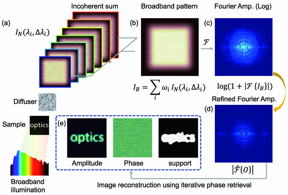
Fig. 1. Principle of single-shot broadband scattering imaging. In the case of a broadband source (a), the broadband pattern (b) is the incoherent spectrally weighted sum of the monochromatic speckle patterns corresponding to all wavelengths present in the source. The size of these monochromatic speckles is geometrically scaled with increasing wavelengths, but the micro-structures are ever-changing. In the presented method, the broadband speckle is first transformed into the Fourier domain (c) and then refined in the complex cepstrum to extract an estimated object Fourier spectrum (d). (e) A modified iterative phase retrieval algorithm is then used to reconstruct the sample, support, and Fourier phase simultaneously.

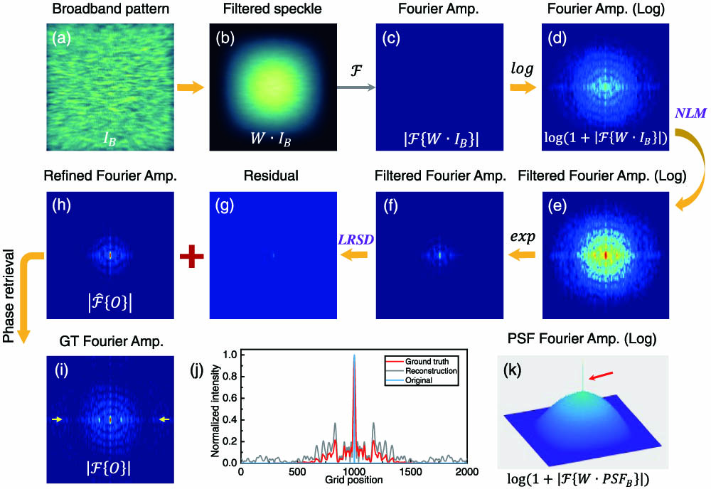
Fig. 2. Noninvasive broadband scattering imaging reconstruction pipeline. The broadband pattern IB (a) is first filtered by a two-dimensional Hanning window to avoid spectrum leakage (b) W·IB and then transformed into the Fourier domain. The Fourier amplitude (c) is reserved and converted into the logarithmic domain (d). The spectrum is filtered by NLM (e) and transmitted back into the Fourier domain (f). A crucial step to remove the peak noise is handed over to the LRSD. After eliminating the sparse part (g), the reserved low rank part (h) is certified as the estimated object spectrum. A modified phase retrieval is then applied on (h) to retrieve the object information. The ground truth object Fourier spectrum is presented in (i). The line profiles (j) along the opposite yellow arrows in (i) show a comparison among the original (c), the ground truth (i), and the recovered spectrum (h). Notably, the recovered spectrum contains richer low-frequency information than the original spectrum. The windowed logarithmic transformed PSF spectrum is shown in (k) with the peak highlighted by a red arrow. NLM, nonlocal means; LRSD, low rank and sparse decomposition.

Fig. 3. Broadband scattering imaging reconstruction pipeline with calibrated PSF. In the OME range, the broadband speckle IB can be treated as the convolution of the object O and the corresponding broadband PSFB. Data acquisition (a) requires a one-time calibration procedure to measure PSFB. Raw captured speckle and the corresponding PSF are background homogenized and filtered by a Gaussian low-pass filter (b) in the frequency domain [(c) and (d)]. The image reconstruction algorithms (e) include cross correlation, nonlinear reconstruction, and our computational reconstruction method. The retrieved four-leaf clover patterns are compared in (f). Artificial cross-section lines are highlighted by gray dashed lines in the nonlinear reconstruction. The normalized intensity of the 76th column along the yellow dotted line in each result (f) is presented in (g). Notably, our method outperforms the other methods, achieving lower background and higher fidelity. GT, ground truth; CC, cross-correlation; NL, nonlinear reconstruction.

Fig. 4. Experimental validation without calibrating PSF with an illumination bandwidth of Δλ/λ=44.8%. (a) Photography of a lithographic letter “B” via lens imaging. Reconstructed results by our method (b), Katz et al. (c), and Wu et al. (d). (e)–(h) Ground truth and the retrieved Fourier phase via the three methods. GT, ground truth. Scale bars are 40 camera pixels in all subgraphs.

Fig. 5. Experimental validation with PSF calibration under broadband illumination (Δλ/λ=44.8%). (a) Photography of a tailored USAF target via lens imaging. Reconstructed results by cross-correlation (b), nonlinear reconstruction with α=0.4, β=0.3 (c), Edrei et al. [34] (d), and our method (e). (f) Line profiles along the yellow arrow in (a) and the same spatial position in each subgraph (b)–(e). GT, ground truth; CC, cross-correlation; NL, nonlinear reconstruction. Scale bars are 40 camera pixels in all subgraphs.

Fig. 6. Comparison of the reconstructions under three different types of broadband illumination calculated from numerical simulation. (a) The normalized spectrum of a femtosecond pulse with FWHM=100  fs pulse width (FWHM=100  nm spectrum). (b) An optical comb with a fixed comb line of 20  nm and the spectrum spanning from 360 nm to 830 nm. (c) The “D65” light source spectrum used to simulate artificial sunlight. (d)–(f) Broadband PSF, speckle, and the recovered objects from both methods (methods A and B) corresponding to each light source in (a)–(c). The broadband PSF autocorrelation patterns are inserted in the bottom left of the first column of (d)–(f). The scale bars in (d)–(f) are 500 camera pixels in the left two columns and 30 camera pixels in the rightmost column.

Fig. 7. Transmission scattering geometry and coordinate. (a) Free space transmission scattering geometry. (b) Incidence and observation directions, (c) k-vectors of the incident light ki, the transmitted light kt, and a k-vector in the observation direction ko.

Fig. 8. Emulation results under different illumination spectral widths. (a) Normalized spectrum profile of illumination bandwidth FWHM varying from Δλ=0  nm to Δλ=104  nm. (b) The autocorrelation intensity profiles of the corresponding broadband PSF patterns with the illumination shown in (a). (c) Neuron cell-like pattern used to generate speckles. (d) Speckle patterns under different illumination in (a). The scale bar is 20 camera pixels in (c) and 300 camera pixels in (d).

Fig. 9. Scattering imaging results under different illumination bandwidths via our proposed method A using simulated data. (a) Ground truth object. (b) Fourier amplitude of (a). (c) Recovered results using speckles under different illumination bandwidths [Fig. 8(d)]. (d) Estimated support regions of (c). (e) Retrieved Fourier amplitude corresponding to (c). (f) Quantitative performance of (c) with (a) as a reference. GT, ground truth. Scale bars are 20 camera pixels in (a), (c), and (d) and 200 camera pixels in (b) and (e).

Fig. 10. Imaging results with quantitative performance under different illumination bandwidths via our proposed method B using simulated data. (a) Ground truth object. (b)–(g) Recovered hidden objects using speckles from Fig. 8(d). GT, ground truth. Scale bars are 20 camera pixels in all subgraphs.

Fig. 11. Experimental setup. A scattering slab is illuminated by a wide-spectrum LED light source with a spectral range from 400 to 1100 nm (FWHM=280  nm). The broadband scrambled patterns are recorded lenslessly by a scientific CMOS camera.

Fig. 12. Experimental comparison of broadband and narrowband illuminated imaging performance via cross-correlation strategy. First column, photography of ground truth objects. Columns 2–5 show imaging results from 220-grit ground glass diffuser with broadband illumination (Δλ=280  nm) and narrowband irradiance centered at λc=530  nm (Δλ=35  nm) and λc=625  nm (Δλ=17  nm), respectively. Columns 6–8 represent imaging results of 600-grit glass diffuser with the same white, green, and red LED illumination. Scale bars are 50 camera pixels in the rightmost column. Performance comparison of the reconstructed object along the lines indicated by the white arrows is shown next to the results.

Fig. 13. Nonlinear reconstruction results of the letter “B” object. The left part corresponds to the retrieved object along different tunable parameters. The right part presents a metric matrix to search for the sharpest image from the left part by using a gradient magnitude based evaluation index. The purple, blue, and green boxes show the reconstruction results with matched, phase-only, and inverse filters, respectively. Results above the yellow dotted line show spurious solutions due to the low power of the power spectrum. The gray and pink boxes indicate the best performance produced by the quality assessment function and from naked eyes. Arrows I and II represent the reconstruction changes by the PSF and the speckle modification, respectively. Arrow III represents the reconstruction changes by a fixed sum of α and β.

Fig. 14. Extended imaging results of method A. (a) Ground truth object “B.” (b)–(d) The recovered letter “B” from red, green, and white light via method A. (e) Ground truth object “star.” (f) Retrieved object “star” under broadband illumination (Δλ/λ=44.8%). (g) Ground truth object “3.” (f) Retrieved object “3” under broadband illumination (Δλ/λ=44.8%). GT, ground truth. Scale bars in all sub-graphs are 40 camera pixels.

Fig. 15. Complex micro-target imaging via proposed method B. (a) The broadband spectrum (orange) with a bandwidth of 44.8% and the narrowband spectrum (red) with a bandwidth of 2.7% and (green) with a bandwidth of 6.6%. (b)–(d) Speckle pattern under red, green, and white illumination, respectively. (e) Ground truth object. The yellow arrows indicate a micro portion with about 10 μm. (f)–(h) The corresponding retrieved objects from (b)–(d) using the 220-grit ground glass diffuser with a 25 μm pinhole. Scale bars are 300 camera pixels in (b)–(d) and 100 μm in (e)–(h).

Fig. 16. Image reconstruction with changing NLM filtering parameters γ via method A. The optimal parameter selection range shrinks slightly with increasing target complexity.

Fig. 17. Results of different parameters. This figure shows the results reconstructed by method B with different parameters. The leftmost image is the ground truth image used in the simulation. The second to fourth columns represent different λ, which is used to control the ℓ1 regularization, while the rows represent different τ, which is used to control the TV regularization term.

Fig. 18. Measurement of the spatial speckle decorrelation as a function of the displacement laterally and longitudinally. (a) and (b) Translational OME range of the 220-grit and 600-grit ground glass, respectively. (d) and (e) Longitudinal OME range of the 220-grit and 600-grit ground glass. (c) and (f) Effective OME range for the two types of ground glass diffusers. All experiments were repeated for three spectral bands: red, green, and white.

Fig. 19. (a)–(d) Monochromatic speckles at λ=500, 510, 520, and 530 nm from numerical simulation. (e)–(h) Cross-correlation between different speckle patterns of (a)–(d) with (a) as the reference speckle. Inserts are enlarged portions of the central correlation peak. Notably, the cross-correlation terms spread with increasing illumination wavelength diversity. (i) Spectral decorrelation of the speckle patterns versus illumination spectral width. Scale bars in (a)–(d) are 50 camera pixels.

Fig. 20. Imaging resolution varies with the size of the pinhole probes. (a)–(c) Recovered results from red, green, and white illuminated patterns using 220-grit ground glass with a 50 μm, 100 μm, and 200 μm pinhole, respectively. (d) Broadband PSF autocorrelation as a function of the pinhole size for each PSF corresponding to (a)–(c). (e) Normalized autocorrelation intensity profiles of all PSFs along the arrow presented in (d). Scale bars are 50 camera pixels in (a)–(c).

Fig. 21. Imaging depth-of-field analysis with a fixed interval δ=2  mm defocus distance. (a)–(c) Imaging results of red, green, and white illuminated at different depths of field under 220-grit ground glass via method B, respectively. The leftmost column indicates the in-focus results with the object and the pinhole at the same spatial position. The right four columns display the defocused results. Scale bars in the rightmost column are 50 camera pixels.

Fig. 22. Anisotropic correlations in broadband speckle patterns. (a) Broadband speckle pattern obtained by numerical simulation. (b) Enlarged border parts I, II, III, and IV of (a). (c) Autocorrelation of different parts in (b). (d) Enlarged central part V and its corresponding autocorrelation. (e)–(h) Real experiment observed broadband speckle and the anisotropic correlation phenomenon from 220-grit ground glass. The scale bars in (a) and (e) are 200 camera pixels.

Fig. 23. Position-dependent broadband speckle memory effect. (a) A typical scrambled pattern under broadband irradiation. (b) and (c) Translation memory effect range of the 600-grit and 220-grit ground glass calculated from different regions. The translation memory effect range is wider for the central part (orange box) than for the boundary part (blue box). The scale bar is 200 camera pixels in (a).

Table 1. Comparison among State-of-the-art Scattering Methods^a

Table 1. Modified phase retrieval algorithm