Lensless imaging through thin scattering layers under broadband illumination

Wei Li; Bingjian Wang; Tengfei Wu; Feihu Xu; Xiaopeng Shao

doi:10.1364/PRJ.466065

Abstract

Lensless scattering imaging is a prospective approach to microscopy in which a high-resolution image of an object is reconstructed from one or more measured speckle patterns, thus providing a solution in situations where the use of imaging optics is not possible. However, current lensless scattering imaging methods are typically limited by the need for a light source with a narrowband spectrum. Here, we propose two general approaches that enable single-shot lensless scattering imaging under broadband illumination in both noninvasive [without point spread function (PSF) calibration] and invasive (with PSF calibration) modes. The first noninvasive approach is based on a numerical refinement of the broadband pattern in the cepstrum incorporated with a modified phase retrieval strategy. The latter invasive approach is correlation inspired and generalized within a computational optimization framework. Both approaches are experimentally verified using visible radiation with a full-width-at-half-maximum bandwidth as wide as 280 nm (

Δ λ / λ = 44.8 %

) and a speckle contrast ratio as low as 0.0823. Because of its generality and ease of implementation, we expect this method to find widespread applications in ultrafast science, passive sensing, and biomedical applications.

Although performing imaging with scattered light is intractable, it has wide applications in many fields, such as biomedical, astronomical, and underwater imaging. This problem is challenging in that the incident wave is randomly modulated by the scattering media, resulting in a disordered pattern containing massive speckle spots. Fortunately, thanks to recent advances in wave front shaping [1 –5], the disordered information can be redistributed and decoded from the observed speckle pattern. For instance, measuring the transmission matrix (TM) allows one to perform focusing [6 –9], as well as imaging [10 –12] or transmitting information [13 –15], through or inside the scattering medium. While, in principle, acquiring TM requires coherent illumination, its extension to broadband case will open fascinating applications in ultrafast science. For this purpose, the TM-based methods are further extended in the spectral domain by accessing the multispectral transmission matrix (MSTM) to cope with polychromatic light. Such techniques have shown success in ultrafast lasers [16 –19] and fiber optics [20]. However, characterizing the scattering medium requires thousands of images captured under vibration isolation conditions, which precludes its applications in dynamic and harsh environments.

A separate approach known as speckle correlation imaging (SCI) also shows promise in broadband focusing and imaging through scattering media [21,22]. This approach relies on persistent correlations, such as the optical memory effect (OME) [23,24], which enables single-shot, high-fidelity, diffraction-limited imaging through scattering media without any prior knowledge of or access to the scattering media. While promising, regular SCI, based on the speckle generated from quasi-monochromatic illumination (typically $< 20 nm$ ), is inherently incompatible with the extremely broad nature of white light spectra. However, the crucial coherence length $L_{c} = λ^{2} / Δ λ$ of the light sources is inversely proportional to the illumination bandwidth $Δ λ$ [25]. Speckle patterns emitted by broadband radiation display low-contrast structures and thus obstruct optical manipulation and inverse reconstruction.

Indeed, the broadband pattern can be thought of as the incoherent superposition of multiple monochromatic speckle patterns produced by the different frequency components encompassed by the light spectrum. Essentially, when observing a speckle pattern, an increase in wavelength (all other parameters remaining fixed) has two effects. First, the observed speckle pattern undergoes a spatial scaling. When the wavelength increases, the speckle pattern expands and vice versa. The second effect is on the random phase shifts imparted to the scattered wave by the surface-height fluctuations $h$ . Since those phase shifts are proportional to $h / λ$ , an increase in wavelength will decrease the random phase shifts and vice versa. When the surface is rough on the scale of a wavelength, phase wrapping into the interval (0, $2 π$ ) will result in changes in the detailed structure of the speckle pattern [26]. For the above two reasons, the extended illumination bandwidth will result in dephasing and speckle aliasing [27], thus reducing the contrast of the observed speckle pattern and further obstructing the reconstruction process.

Sign up for Photonics Research TOC. Get the latest issue of Photonics Research delivered right to you！Sign up now

As different spectral components generate different speckles, current approaches are highly sensitive to the spectral bandwidth. The monochromatic treatment is, therefore, only valid as long as the bandwidth of the source is contained within this spectral correlation bandwidth. Extending narrowband to broadband light can effectively ease the trade-off between the filter bandwidth and detection signal-to-noise ratio (SNR). Furthermore, it can potentially help increase the penetration depth, which is critical for biomedical fields, including neuroscience.

To mitigate the constraint of the narrowband operation, several imaging techniques have been developed. A straightforward method is based on spectral components such as spectral filters [28], prisms [29], or even scattering-assisted spectrometers [30] to resolve broadband spectra into well-separated spectral channels. This improves the speckle contrast as well as the performance of object retrieval. Although these methods have proven efficiency, the trade-off between spectral resolution and spectral range can limit their performance. Moreover, imposing spectral filters on broadband sources leads to a dramatic reduction in flux, which may be impractical in some applications. The ability to use the full-flux of low-flux ultra-broadband sources, such as table-top high-harmonic generation (HHG) systems [31], could provide a breakthrough for practical imaging applications. Incoherent scattering imaging can also rely on deep learning modules [32]. Nevertheless, the price to pay is a fuzzy physical model and a large training dataset. To date, controlling scattered light for deep focusing under broadband illumination has attracted much attention [16 –19,33]. However, the necessary scattering imaging methods combining broadband illumination with diffraction-limited spatial resolution are currently lacking. These representative state-of-the-art scattering imaging methods, as well as the effective illumination bandwidth, are summarized in Table 1.Table 1.

Comparison among State-of-the-art Scattering Methods^a

Method	Bandwidth (FWHM)	Captured Frames	Precision Calibration	Object Sparse Constraint	Image Fidelity
Bertolotti et al. [21]	40 nm	Multi-shot	W	W/O	High
Katz et al. [22]	20 nm	Single-shot	W/O	W	High
Edrei et al. [34]	1 nm	Single-shot	W	W/O	High
Wu et al. [35]	1 nm	Single-shot	W/O	W	High
Badon et al. [16]	13.8 nm	Multi-shot	W	W/O	Moderate
Li et al. [29]	60 nm	Single-shot	W	W	High
Divitt et al. [36]	200 nm	Multi-shot	W	W	Moderate
Lu et al. [37]	200 nm	Single-shot	W/O	W	Moderate
Ours (A)	280 nm	Single-shot	W/O	W	High
Ours (B)	280 nm	Single-shot	W/O	W/O	High

$W = with$ , $W / O = without$ . $A = Method$ A, $B = Method$ B.

In this paper, we propose two individual methods for realizing scattering imaging under broadband illumination using only a single speckle measurement under noninvasive and invasive conditions. The major difference between invasive and noninvasive methods is that invasive methods pre-calibrate point spread function (PSF) information for scattering systems, whereas noninvasive methods require no a priori information about the medium or its properties. In contrast to previous approaches, both methods neither require any spectral filters, nor have additional assumptions on the spectral content of the signals. In the noninvasive approach (method A), we extract the object Fourier spectrum from the broadband pattern by using a cepstrum shaping method combined with a matrix decomposition strategy. We show that by unique computational processing, the lost low-frequency information can be reproduced in the Fourier domain. After applying a modified phase retrieval procedure, sharp reconstruction results can be achieved even with a speckle contrast ratio (SCR) as low as 0.0823 [26]. The invasive approach (method B) is based on an optimization framework to solve a general de-correlagraphy problem. The proposed computational framework can effectively reduce the background level of the recovered image, while preserving sharp edges and high-frequency features. Experimental validations under the 280 nm illumination spectrum spanning the visible region show the applicability of both methods. Our approach enables imaging through scattering media under broadband radiation, which we expect to make much more efficient use of such state-of-the-art light sources as third-generation synchrotrons and table-top HHG sources for operating in heavily scattering environments. Moreover, the capability to treat broadband light can also empower the fields of florescence imaging, night vision detection, and passive sensing.

For simplicity, our problem discussion is limited to the scope of the OME region. The recorded broadband speckle $I_{B}$ can be described by the convolution between the broadband PSF, ${PSF}_{B}$ , and the object function, $O$ , $I_{B} = O * {PSF}_{B} + N,$ (1)where the symbol “ $*$ ” denotes a two-dimensional convolution operation, $N$ represents the noise, and the subscript $B$ represents the broadband illumination. By employing the convolution theorem [21,38], the autocorrelation of the broadband pattern $I_{B}$ yields $I_{B} ⋆ I_{B} \approx (O ⋆ O) * ({PSF}_{B} ⋆ {PSF}_{B}),$ (2)where the symbol “ $⋆$ ” represents a two-dimensional correlation operation. The omitted $(O * {PSF}_{B}) ⋆ N$ term is due to the statistically uncorrelated between the noise term N and the PSF_B. The autocorrelation of noise can be approximated as a constant background [22]. When dealing with a narrowband illumination case, the autocorrelation of PSF can be simplified as a Dirac delta function and omitted [26]. However, this assumption does not hold for broadband illumination as the autocorrelation of the broadband pattern gathers $M$ terms monochromatic speckles autocorrelation and $C_{M}^{2}$ terms cross-correlation between speckles of different wavelengths in spectrum discretization.

Let us assume that the broadband spectrum light source $Q (λ, Δ λ)$ can be regarded as a linear superposition of multiple narrowband spectrum light sources $Q_{i} (λ_{i}, Δ λ_{i})$ $(i = 1, 2, \dots, M)$ with each one under the narrowband illumination hypothesis. Here, $λ$ and $λ_{i}$ represent the central wavelength of the broadband and each narrowband light, and the bandwidths of the broadband and narrowband light are denoted by $Δ λ$ and $Δ λ_{i}$ , respectively. Considering the broadband illumination case, the broadband PSF, ${PSF}_{B} (λ, Δ λ)$ can be expressed as ${PSF}_{B} (λ, Δ λ) = \sum_{i = 1}^{M} ω_{i} {PSF}_{N} (λ_{i}, Δ λ_{i}),$ (3)where $ω_{i}$ denotes the weight coefficient of each spectral component, and the subscript $N$ represents narrowband illumination. Correspondingly, the autocorrelation of the broadband speckle pattern can be written as ${PSF}_{B} (λ, Δ λ) ⋆ {PSF}_{B} (λ, Δ λ) = \sum_{i = 1}^{M} ω_{i}^{2} {PSF}_{N} (λ_{i}, Δ λ_{i}) ⋆ {PSF}_{N} (λ_{i}, Δ λ_{i}) + \sum_{i = 1}^{M} \sum_{j \neq i}^{M} ω_{i} ω_{j} {PSF}_{N} (λ_{i}, Δ λ_{i}) ⋆ {PSF}_{N} (λ_{j}, Δ λ_{j}) .$ (4)

From Eq. (4), the autocorrelation of the broadband speckle can be separated into two parts. The first term incorporates a superposition of all autocorrelation parts, whereas the latter term accounts for contributions from all cross-correlation parts. Considering the discussions in Ref. [38] and supposing the imaging system has a circle pupil, the first part of the broadband PSF’s autocorrelation can be further expressed as $\sum_{i = 1}^{M} ω_{i}^{2} {PSF}_{N} (λ_{i}, Δ λ_{i}) ⋆ {PSF}_{N} (λ_{i}, Δ λ_{i}) \propto \sum_{i = 1}^{M} ω_{i}^{2} [1 + {| 2 \frac{J_{1} (π D r / λ_{i} z)}{π D r / λ_{i} z} |}^{2}],$ (5)where $J_{1} (\cdot)$ denotes the first kind of Bessel function of the first order. $D$ , $r = \sqrt{{(Δ x)}^{2} + {(Δ y)}^{2}}$ with $r = (x, y)$ on observation plane, and $z$ are the pupil size, the radius of two-dimensional polar coordinate in image plane, and the image distance, respectively. The contribution of the first part is to form a peak-to-background ratio (PBR) of 2:1 spike in the autocorrelation pattern, while the second part can be calculated as $\sum_{i = 1}^{M} \sum_{j \neq i}^{M} ω_{i} ω_{j} {PSF}_{N} (λ_{i}, Δ λ_{i}) ⋆ {PSF}_{N} (λ_{j}, Δ λ_{j}) \propto \sum_{i = 1}^{M} \sum_{j \neq i}^{M} ω_{i} ω_{j} {1 + \exp [- σ_{h}^{2} (n - 1) | k_{i} - k_{j} |] \times {2 \frac{J_{1} (π D r / {\bar{λ}}_{i j} z)}{π D r / {\bar{λ}}_{i j} z} * F {\exp [\frac{j (k_{i} - k_{j}) r^{' 2}}{2 z}]}}^{2}},$ (6)where $σ_{h}$ and $n$ denote the height standard deviation and the refractive index of the scattering media, respectively. $F {\cdot}$ indicates the Fourier transform, and $r^{'} = (ξ, η)$ are the coordinates of the plane just to the right of the scattering surface. $k$ denotes the wave vector, $k = 2 π / λ$ . The newly involved wavelength term ${\bar{λ}}_{i j}$ represents the average values of $λ_{i}$ and $λ_{j}$ . The residual background term accumulated by the second part [Eq. (4)] increases gradually as the wavelength difference increases. See Appendix D for details. Substituting Eqs. (5) and (6) to Eq. (4), we eventually derive the autocorrelation of the broadband PSF (refer to Appendix A for detailed derivation).

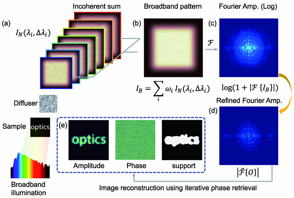
A radiation beam consisting of multiple wavelengths is illuminated on the sample and the exiting field is scattered by an off-the-shelf diffuser to form broadband pseudorandom patterns, which is the incoherent superposition of speckle patterns of each wavelength [see Figs. 1(a) and 1(b)]. To reconstruct the object, $O$ , from the single-shot measured image $I_{B}$ , we need to solve the ill-conditioned inverse scattering problem by utilizing phase retrieval. However, as discussed in Section 2, the autocorrelation of the broadband ${PSF}_{B}$ no longer satisfied the delta function approximation and thus caused the failure of the SCI method. Novel methods are highly desired to remedy this issue. Here, based on experimentally observed similarities in the Fourier spectra of objects and speckles and inspired by homomorphic filtering, we propose a spectrum refinement principle that enables the extraction of the pure object Fourier spectrum from the caustic broadband pattern Fourier spectrum. The Fourier spectrum extraction procedure is depicted in Fig. 2. The phase retrieval is then performed using the refined Fourier spectrum pattern [see Fig. 1(d)] as input into a hybrid relaxed averaged alternating reflections (RAAR) [39] and hybrid input and output (HIO) [40,41] algorithm, with a shrink-wrap-like support update [42] (see Algorithm 1 for details). The object, support region, and Fourier phase can be retrieved simultaneously [Fig. 1(e)].

Figure 1.Principle of single-shot broadband scattering imaging. In the case of a broadband source (a), the broadband pattern (b) is the incoherent spectrally weighted sum of the monochromatic speckle patterns corresponding to all wavelengths present in the source. The size of these monochromatic speckles is geometrically scaled with increasing wavelengths, but the micro-structures are ever-changing. In the presented method, the broadband speckle is first transformed into the Fourier domain (c) and then refined in the complex cepstrum to extract an estimated object Fourier spectrum (d). (e) A modified iterative phase retrieval algorithm is then used to reconstruct the sample, support, and Fourier phase simultaneously.

Figure 2.Noninvasive broadband scattering imaging reconstruction pipeline. The broadband pattern

I_{B}

(a) is first filtered by a two-dimensional Hanning window to avoid spectrum leakage (b)

W \cdot I_{B}

and then transformed into the Fourier domain. The Fourier amplitude (c) is reserved and converted into the logarithmic domain (d). The spectrum is filtered by NLM (e) and transmitted back into the Fourier domain (f). A crucial step to remove the peak noise is handed over to the LRSD. After eliminating the sparse part (g), the reserved low rank part (h) is certified as the estimated object spectrum. A modified phase retrieval is then applied on (h) to retrieve the object information. The ground truth object Fourier spectrum is presented in (i). The line profiles (j) along the opposite yellow arrows in (i) show a comparison among the original (c), the ground truth (i), and the recovered spectrum (h). Notably, the recovered spectrum contains richer low-frequency information than the original spectrum. The windowed logarithmic transformed PSF spectrum is shown in (k) with the peak highlighted by a red arrow. NLM, nonlocal means; LRSD, low rank and sparse decomposition.

After we measure the broadband pattern $I_{B}$ [Fig. 2(a)], we first filter it with a two-dimensional Hanning window in real space $W \cdot I_{B}$ [Fig. 2(b)] to avoid spectrum leakage and then transform it into the Fourier domain [see Fig. 2(c) for Fourier amplitude]. The part of the Fourier phase corrupted by scattering is discarded, which is not shown here. We note, first, that the Fourier spectrum is sparse, as the energy of the power spectrum is concentrated around zero frequency [see the blue line profile in Fig. 2(j)], which necessitates an approach to retrieval. To avoid oscillations caused by near zero values in the spectrum, we add an all-one matrix on the Fourier amplitude and then convert it into the logarithmic domain [Fig. 2(d)]. Notably, more details and noise in the spectrum are highlighted with logarithmic transform; therefore, a smooth filter via nonlocal means (NLM) [43] is applied to exclude the noisy profile introduced by the broadband ${PSF}_{B}$ [see the hemispherical surface attached burrs in Fig. 2(k)]. The size of the patch and research window of the NLM are set as 5 and 11, respectively, and the smooth parameter $γ$ is set as 3. As $γ$ controls the decay process of the Gaussian function in NLM, a higher value of $γ$ is suitable for a relatively simple target to obtain a smoother spectrum and vice versa. Detailed parameter selection rules are arranged in Appendix C.

The filtered spectrum is then transformed back into the Fourier domain [Fig. 2(f)]. The next step involves a low-rank and sparse decomposition (LRSD) procedure [44] based on robust principal component analysis (RPCA) [45] to remove the residual peak noise caused by the broadband ${PSF}_{B}$ [highlighted with a red arrow in Fig. 2(k)]. We classify this peak noise into a sparse part according to its sparse property [Fig. 2(g)], and the low-rank part represents the final separated Fourier spectrum [Fig. 2(h)]. The ground truth object Fourier spectrum is presented in Fig. 2(i). Note that the low-frequency information reappears in the Fourier domain after processing [see the comparison in Figs. 2(c), 2(h), and 2(i)]. The central line along the two opposite arrows of Figs. 2(c), 2(h), and 2(i) depicted by gray, red, and blue lines also verified the effectiveness of the proposed method, for richer low-frequency information and higher cut-off frequency.

Finally, we obtain the refined Fourier spectrum $| \hat{F} {O} |$ [Fig. 2(h)], and in the next step, we perform phase retrieval to reconstruct the target information. However, as the broadband ${PSF}_{B}$ information is unknown, object spectrum recovery is an ill-conditioned problem; therefore, robust phase retrieval is needed to remedy this issue. Here, we modified the iterative alternating projection method by introducing an adaptive support region and a hybrid phase retrieval strategy. Specifically, the iteration was carried out using a combination of the RAAR and HIO algorithms, with a shrink-wrap-like support update. We calculate the root mean square error (RMSE) between the refined Fourier amplitude and the Fourier amplitude generated by the estimated object in each iteration. We chose typically 80 iterations to ensure that the RMSE of the RAAR algorithm converged to $< 0.05$ . The subsequent HIO algorithm is used for smearing out the background noise and 10 iterations are typically adequate to obtain the final result. The feedback parameter $β$ is set as $β_{1} = β_{2} = 0.8$ for both the RAAR and HIO algorithms. Accompanied by the iteration, the adaptive support region is controlled by an alternative convolution with a Gaussian kernel (Algorithm 1, step 6) and a threshold operation (Algorithm 1, step 7), which act as dilation and erosion. As the iterative number increases, this exported support region will change from a loose size to a tight one (Algorithm 1, steps 2-7). The initial $σ^{(0)} = 3 ϵ$ , where $ϵ$ represents the pixel size related to the imaging sensor. It is worth emphasizing that we selected a non-centrosymmetric support $S_{0}$ , for instance, an equilateral triangle, as an initial support. Using a non-centrosymmetric support region considerably speeds up convergence and effectively avoids the twin-image problem.

To explain how the process works in greater detail, four projection operations are defined. The projection operations $P_{s}$ , $P_{m}$ , $R_{s}$ , and $R_{m}$ project points in two sets, $S$ (support) and $M$ (modulus) [46]. When the image belongs to both sets simultaneously, we reach an equivalent solution. The support projector $P_{s}$ involves setting to 0 the components outside the support, while leaving the rest of the values unchanged. $P_{s} ρ (r) = {\begin{matrix} ρ (r) & if r \in S \\ 0 & otherwise \end{matrix},$ (7)where $ρ (r)$ denotes the object intensity distribution, with $r$ being the coordinates in the object (or real) space. The role of modulus projector $P_{m}$ is to set the modulus to the measured one $m (k) = \sqrt{I (k)}$ in the reciprocal space, and leaving the phase unchanged: $P_{m} \tilde{ρ} (k) = P_{m} | \tilde{ρ} (k) | e^{i φ (k)} = m (k) e^{i φ (k)} .$ (8)

The reflectors of the support projector $P_{s}$ and modulus projector $P_{m}$ are defined as, $R_{s} = 2 P_{s} - I$ and $R_{m} = 2 P_{m} - I$ , respectively.

According to the notation above, the recursive form of HIO algorithm would be $ρ^{(n + 1)} (r) = [P_{s} P_{m} + P_{\underline{s}} (I - β P_{m})] ρ^{(n)} (r)$ (9)with $P_{\underline{s}} = (I - P_{s})$ the complement of the projector $P_{s}$ . Similarly, the RAAR algorithm can be written as $ρ^{(n + 1)} (r) = [\frac{1}{2} β (R_{s} R_{m} + I) + (1 - β) P_{m}] ρ^{(n)} (r) .$ (10)

For clarity, we describe our modified phase retrieval procedure in Algorithm 1.Algorithm 1.

Modified phase retrieval algorithm

Input: initial solution

ρ^{(0)}

, initial support

S_{0}

, initial standard deviation of the Gaussian kernel

σ^{(0)}

, RAAR iteration times

N_{1}

and the feedback constant

β_{1}

, HIO iteration times

N_{2}

and the feedback constant

β_{2}

, RAAR start iteration counter

i \leftarrow 1

, HIO start iteration counter

j \leftarrow 1

, support region update symbol

m

Output: recovered object

\hat{ρ}

, estimated support

\hat{S}

, recovered Fourier phase

angle {\hat{F} (ρ)}

1: while

i \leq N_{1}

2: if

\mod (i, m) = 0

then

σ^{(i)} = \min (0.99 σ^{(i - 1)},0.5 σ^{(0)})

4: else

σ^{(i)} = σ^{(i - 1)}

S_{i} = S_{i - 1} * \exp (- r^{2} / 2 {(σ^{(i)})}^{2})

S_{i} \leftarrow S_{i} \times (S_{i} \geq \max (0.15 S_{i}))

ρ^{(i + 1)}

← solution of Eq. (10).

i \leftarrow i + 1

10: while

j \leq N_{2}

11: Repeat step 2-step 7 for each

j

12:

ρ^{(j + 1)}

← solution of Eq. (9).

13:

j \leftarrow j + 1

14: return

\hat{ρ} = ρ^{(N_{2})}

\hat{S} = S_{N_{2}}

angle {\hat{F} (ρ)} = angle {F (\hat{ρ})}

In the present method, phase retrieval is a standalone step that depends solely on the refined spectrum. It can also be integrated as a module in algorithms for other types of lensless imaging (coherent diffraction imaging, holography, ptychography) to allow them to cope with broadband sources.

Figure 3 presents the data acquisition and reconstruction process with PSF calibration. An object and a pinhole are alternatively placed at the same spatial position in the optical configuration (see details in Appendix C), which captures the broadband speckle, $I_{B}$ , and the corresponding PSF, ${PSF}_{B}$ . The raw captured speckle and PSF are then lowpass filtered in the frequency domain (a typical filter length is 15) to eliminate the non-uniform illumination background. Then, we apply a two-dimensional Gaussian lowpass filter of size [2 2] with standard deviation $σ = 0.5$ in the real space to further smooth the pattern.

Figure 3.Broadband scattering imaging reconstruction pipeline with calibrated PSF. In the OME range, the broadband speckle

I_{B}

can be treated as the convolution of the object

O

and the corresponding broadband

{PSF}_{B}

. Data acquisition (a) requires a one-time calibration procedure to measure

{PSF}_{B}

. Raw captured speckle and the corresponding PSF are background homogenized and filtered by a Gaussian low-pass filter (b) in the frequency domain [(c) and (d)]. The image reconstruction algorithms (e) include cross correlation, nonlinear reconstruction, and our computational reconstruction method. The retrieved four-leaf clover patterns are compared in (f). Artificial cross-section lines are highlighted by gray dashed lines in the nonlinear reconstruction. The normalized intensity of the 76th column along the yellow dotted line in each result (f) is presented in (g). Notably, our method outperforms the other methods, achieving lower background and higher fidelity. GT, ground truth; CC, cross-correlation; NL, nonlinear reconstruction.

After preprocessing, we introduce two types of reconstruction algorithms. The first algorithm is based on the cross-correlation strategy: $\hat{O} = I_{B} ⋆ {PSF}_{B} = F^{- 1} [F (I_{B}) \cdot \bar{F ({PSF}_{B})}] .$ (11)

Here $F^{- 1} {\cdot}$ represents the inverse Fourier transform, and the bar above the variable represents a complex conjugate. Inspired by the interferenceless coded aperture correlation holography [47], a modified approach of the cross-correlation method is referred to as the nonlinear reconstruction process: $\hat{O} = F^{- 1} [{| F (I_{B}) |}^{α} \cdot {| F ({PSF}_{B}) |}^{β} \cdot e^{i (φ_{I_{B}} - φ_{{PSF}_{B}})}],$ (12)where $φ_{I_{B}}$ and $φ_{{PSF}_{B}}$ denote the Fourier phase of $I_{B}$ and ${PSF}_{B}$ , respectively. The adjustable parameter $α$ and $β$ are chosen to tune the power spectrum of the object and reconstructing functions, respectively. The advantageous effect of using nonlinear processing has already been observed in Refs. [47,48]. A detailed investigation of this point can be found in Appendix C.

Mathematically, broadband scattering imaging can also be formulated as the following forward model: $g = H (f) + e,$ (13)where $f \in R^{N \times N}$ represents the hidden object, $g \in R^{N \times N}$ is the measurement, $H (\cdot)$ is the mapping of the hidden object to the measurement, and $e \in R^{N \times N}$ denotes the noise components. In our framework, the reconstruction task is accomplished by solving an optimization problem with a joint $ℓ_{1}$ and total variation (TV) regularization under a nonnegative constraint: $\hat{f} = \arg \min_{f \geq 0} \frac{1}{2} {∥ g - H (f) ∥}_{2}^{2} + τ {∥ f ∥}_{TV} + λ {∥ f ∥}_{1},$ (14)where ${∥ \cdot ∥}_{p}$ for $p = 1$ , 2 or TV is the $ℓ_{1}$ -norm, $ℓ_{2}$ -norm or TV-norm, respectively. The parameters ( $τ$ and $λ$ ) are used to control the TV and $ℓ_{1}$ -norm to balance noise removal and object sparsity. Detailed rules for parameters selection are arranged in Appendix C. Here, we use the anisotropic TV norm ${∥ \cdot ∥}_{TV}$ , ${∥ f ∥}_{TV} = \sum_{i} (| {[D_{x} (f)]}_{i} | + | {[D_{y} (f)]}_{i} |),$ (15)where the operators $D_{x} (\cdot)$ , $D_{y} (\cdot)$ are the forward finite difference operators along the horizontal and vertical directions, respectively. The main advantage of this model is that it recovers edges well and removes noise, avoiding the ringing effect.

We develop an iterative inverse algorithm, modified from sparse Poisson intensity reconstruction algorithms theory and practice (SPIRAL-TAP) [49], to obtain an approximate solution of the inverse problem in Eq. (14). Here, in our case, the forward model matrix $H$ is defined as a function called $H (\cdot)$ and the adjoint of $H (\cdot)$ is specified as $H^{T} (\cdot)$ , which denotes the back-projection process. Contrary to the previous deconvolution approaches, the forward and backward models are modified with the cross-correlation [Eq. (11)] and nonlinear reconstruction operation [Eq. (12)], respectively. The adjustable parameters are set the same as in nonlinear reconstruction ( $α = 0.4$ and $β = 0.3$ ). The SPIRAL-TAP approach for the de-correlagraphy problem will consider the iterations to be sufficiently close to the optimal solution if ${‖ {\hat{f}}_{k + 1} - {\hat{f}}_{k} ‖}_{2} / {‖ {\hat{f}}_{k} ‖}_{2} \leq ε,$ (16)where $ε$ is some small constant, the subscript $k$ denotes the $k$ -th iteration. In our algorithm, the stopping criterion is satisfied when $ε \leq 10^{- 6}$ .

Some artifacts from the recovery process nevertheless deserve attention; for instance, the abnormal cross-section lines indicated by gray dashed lines in the nonlinear reconstruction [Fig. 3(f)]. These cross-section lines come from the noninteger power transformation of the spectrum in the nonlinear reconstruction, resulting in a simultaneous increase in detail and high-frequency noise, unavoidably producing these artifacts. As these adjustable parameters $α$ and $β$ decrease, the resolution of the reconstruction will improve moderately, while the noise will increase dramatically. (Details about this point can be found in Appendix C.) However, thanks to the regularized inversion method, these artifacts are not dominant in the recovered pattern [see the comparison in Fig. 3(f)]. In addition, the differences between the values of points a and b are 1, 0.6, 0.68, and 0.75, respectively [Fig. 3(f)]. Reconstructions of the proposed method have sharp boundaries and contain very little noise. A typical reconstruction requires at least four iterations. Solving for $1800 \times 1800 = 3.24$ million pixels takes 10.35 s (2.59 s per iteration) on a dual-core computer and with a GeForce RTX 2080 Ti GPU. Moreover, for further algorithm acceleration, this fused lasso problem can also be solved by the alternating direction method of multipliers (ADMM) [50] or fast iterative shrinkage-thresholding algorithm (FISTA) [51], which will be exploited in the future.

Experimental validation. The single-shot method A was validated in the visible domain on a broadband and spatially incoherent source with its spectrum full-width at half-maximum ( $FWHM = 280 nm$ ). Then, method B was tested under the same experimental conditions with additional PSF information. The objects employed for these experiments are ubiquitous in the field of scattering imaging and allow for algorithmic validation and resolution estimation.

A lens imaged lithographic letter “B” is shown in Fig. 4(a). The experiment was performed using a commercial broadband light emitting diode (LED) (Thorlabs, MBB1L3, wavelength range of 400–1100 nm, $FWHM = 280 nm$ ). The collimated light is incident on the object and then transmitted 24 cm to the diffuser (Edmund, 45-656). The light scattered from the diffuser was recorded by a scientific complementary metal oxide semiconductor (sCMOS) camera (Pco.edge. 4.2, pixel size 6.5 μm) set at 12 cm from the diffuser. Further details on the experimental setup can be found in Appendix C.

Figure 4.Experimental validation without calibrating PSF with an illumination bandwidth of

Δ λ / λ = 44.8 %

. (a) Photography of a lithographic letter “B” via lens imaging. Reconstructed results by our method (b), Katz et al. (c), and Wu et al. (d). (e)–(h) Ground truth and the retrieved Fourier phase via the three methods. GT, ground truth. Scale bars are 40 camera pixels in all subgraphs.

Our single-shot method was then applied to the broadband pattern, at the center of mass of the broadband spectrum $λ_{c} = 625 nm$ ( $Δ λ / λ = 44.8 %$ ). Two other state-of-the-art single-shot methods were also introduced for comparison. The SCI method pioneered by Katz et al. performs phase retrieval on speckle autocorrelation. For each loop, the HIO algorithm [41] was run with a decreasing $β$ factor from $β = 2$ to $β = 0$ , in steps of 0.04. For each $β$ value, 30 iterations of the HIO algorithm were performed. The obtained result was fed as an input to additional 30 iterations of the “error reduction (ER)” algorithm to obtain the final result. The second reconstruction method in comparison from bispectrum analysis [35] utilizes the phase closure theory to extract the phase information from subblock speckles, in which the phase is projected onto 18 uniformly spaced angles from (0, $2 π$ ). Moreover, the time costs of the reconstruction of speckle sizes of $1800 \times 1800 = 3.24$ million pixels are listed at the bottom of Fig. 4. The experiments were all performed with MATLAB 2018b in Windows 10 running on a dual-core chip Intel Core i9-10900K and 128G memory.

Apparently, both methods [Figs. 4(c) and 4(d)] failed to reconstruct the object and the corresponding Fouier phase under broadband illumination. From the correlation perspective, the failure of the speckle correlation is attributable to the fact that the autocorrelation of broadband PSF cannot be approximated as a delta function, as described in Eq. (6) and mentioned in Fig. 1. Therefore, the estimation of object autocorrelation is stained and further obstructs phase retrieval. The statistical noise of the bispectrum is higher than the autocorrelation, so more speckle spots are required in reconstruction, making it difficult to cope with low-contrast broadband patterns. The proposed method successfully reconstructs the target information, where the PSNR value is as high as 22.63 dB. The similarity between the object Fourier phase and the reconstructed result [see Figs. 4(e) and 4(f)] is obvious.

It is worth emphasizing that iterative phase retrieval algorithms are highly sensitive to the initial guess, the support constraint, and the convergence criterion. The twin-image problem will interfere with the direction selection in the iterative process, causing the phase retrieval algorithm to wander left and right and unable to quickly jump out of the local minimum. Thus the tuning rules are very general and require experiments during a trial and error method.

Here, thanks to the initial non-centrosymmetric support region estimation, adaptive shrink-wrap strategy, and hybrid retrieval method, we achieve a reconstruction accuracy as high as 85%. The empirical probability of success is an average over 1000 trials, in each of which we generate new random matrices as the algorithm input. We declare that a trial is successful if the SSIM between the ground truth and the reconstruction is $> 0.8$ (see Visualization 1 for a dynamic reconstruction process). Therefore, verifying our approach is highly repeatable and stable. Our method can effectively avoid brute force manual post-selection and considerably increase the reconstruction fidelity. In terms of algorithm time consumption, although our method has the longest reconstruction time, the performance of our results is the best. In algorithm processing, 90% of the time is occupied on NLM filtering, $> 9 %$ of the time is spent on LRSD, and $< 1 %$ is spent on phase retrieval. Subsequent research can integrate the algorithm in the graphics processing unit (GPU) or on the field programmable gate array (FPGA) to increase the processing speed, and it is anticipated to achieve high-speed processing.

The main reconstruction comparison between different state-of-the-art approaches is presented in Fig. 5. A tailored USAF1951 target (Edmund, 55-622) with group 0 element 3-5 is selected as the ground truth object. The broadband PSF is measured with a 100 μm pinhole in the same spatial position of the object. The reconstructed results by different algorithms, including the cross-correlation, nonlinear reconstruction, Edrei et al. [34], and our computational reconstruction method, are shown in Figs. 5(b)–5(e), respectively.

Figure 5.Experimental validation with PSF calibration under broadband illumination (

Δ λ / λ = 44.8 %

). (a) Photography of a tailored USAF target via lens imaging. Reconstructed results by cross-correlation (b), nonlinear reconstruction with

α = 0.4

β = 0.3

(c), Edrei et al. [34] (d), and our method (e). (f) Line profiles along the yellow arrow in (a) and the same spatial position in each subgraph (b)–(e). GT, ground truth; CC, cross-correlation; NL, nonlinear reconstruction. Scale bars are 40 camera pixels in all subgraphs.

As indicated, all methods find the object pattern correctly. Our reconstruction matches perfectly with the ground truth, with PSNR further increasing to 18.57 dB, higher than that of the nonlinear algorithm (15.36 dB). We compare in Fig. 5(f) the intensity profiles along the line indicated by the yellow arrow [see Fig. 5(a)] in each subgraph. Benefiting from the constraint of the $ℓ_{1}$ regular term, our results show a significant difference between the target and background. The use of TV regularization effectively reduces the background level and compensates for the artificial traces caused by power spectrum modulation [see Figs. 3(f) and 5(c)]. It is shown that our reconstruction has the smallest background while keeping the highest image contrast. The hollow numbers “4” and “5” close to the edge of the resolution target are also preserved.

An alternative reconstruction is from the Lucy–Richardson deconvolution algorithm under 400 iterations [52] [Fig. 5(d)]. Due to the inherent linear convolution model, the deconvolution algorithm can produce an acceptable result [see Fig. 5(d)]. Correlagraphy-based reconstructions [Figs. 5(b) and 5(c)] also show clear and sharp-edged results with high reconstruction speed. The effects of background noise and artifacts are well compensated by our improved method [Figs. 5(e) and 5(f)]. This comparison also reveals that the correlation-based methods {with Fig. 5(e) or without regularization [Figs. 5(b) and 5(c)]} do not require precise optical calibration while performing well in broadband scattering imaging [53].

In addition, the memory complexity of our method is $O (N^{2})$ , and the time complexity of each iteration is $O (N^{2} \log N)$ . Although the cost time is slightly longer when processing on the CPU (see Fig. 5), it can be dramatically shortened by using parallel computation on GPU (approximately 10 s for four typical iterations on GeForce RTX 2080 Ti). Further comparisons of different approaches under narrowband and broadband illumination are arranged in Appendices B to E.

Due to the temporal and spectral reciprocity, ultrafast sources can also produce equivalent broadband spectra. Naturally, our method can be used as a plug-and-play image restoration in ultrafast science and passive sensing. To demonstrate this point, we show here a comparison among three types of used scientific broad-spectrum light sources and our methods feasibility from numerical simulation. Figure 6(a) illustrates a transform-limited femtosecond pulse $Δ t Δ ω \sim 1$ with a 100 fs pulse width. The corresponding spectrum ranges from 480 nm to 720 nm, and $FWHM = 100 nm$ ( $Δ λ / λ = 16.7 %$ ). The second revolutionary broadband source is an optical frequency comb with a fixed comb $line o f 20 nm$ and a spectrum ranging from 360 nm to 830 nm. The normalized spectrum of the optical comb is shown in Fig. 6(b) with each comb teeth spectrum $FWHM = 1 nm$ . The third broadband source is the “D65” illumination [see the spectrum in Fig. 6(c)], which is commonly used to simulate artificial sunlight ( $Δ λ / λ = 39.7 %$ ). The broad-spectrum PSFs and speckles generated by these three light sources, and the corresponding imaging results via methods A and B are shown in Figs. 6(d)–6(f), respectively.

Figure 6.Comparison of the reconstructions under three different types of broadband illumination calculated from numerical simulation. (a) The normalized spectrum of a femtosecond pulse with

FWHM = 100 fs

pulse width (

FWHM = 100 nm

spectrum). (b) An optical comb with a fixed comb line of

20 nm

and the spectrum spanning from 360 nm to 830 nm. (c) The “D65” light source spectrum used to simulate artificial sunlight. (d)–(f) Broadband PSF, speckle, and the recovered objects from both methods (methods A and B) corresponding to each light source in (a)–(c). The broadband PSF autocorrelation patterns are inserted in the bottom left of the first column of (d)–(f). The scale bars in (d)–(f) are 500 camera pixels in the left two columns and 30 camera pixels in the rightmost column.

All three broadband speckles produce high-fidelity results with both methods. Intriguingly, our noninvasive method (method A) performs similarly to the invasive method (method B). A possible explanation for this behavior could be the noise-suppressing properties of the NLM method used in cepstrum filtering. Further discussion of the speckle contrast and the imaging performance changes with spectral spread is arranged in Appendix B.

While both methods A and B provide promising solutions to the lensless broadband scattering imaging problem, the hidden scenes are restricted to two-dimensional planar objects and the effective field-of-view still lies in the OME scope. For method A, recovering the high-frequency features of the spectrum remains a great challenge as the complete scattering degradation process is unknown. As a result, this noninvasive method cannot be used to image dense and connected samples. This is also a limitation that applies to all existing statistical-based scattering imaging methods, including method A. For method B, there is a trade-off between the detail of the reconstruction and the degree of denoising owing to the introduction of the TV regularity term. Moreover, the complexity of the algorithm needs to be further reduced. We believe that these drawbacks will be overcome in the future.

With respect to improving imaging performance and capability on challenging scenarios, the next step is to implement our method on a complex 3D scene by leveraging the stereo vision [54] or light field solutions [55]. Higher-fidelity reconstruction is anticipated by applying deep learning modules or scattering matrix inversion to unveil the detailed scattering process. Benefiting from the single-shot data acquisition strategy, future works can also be expanded to the dynamic scattering region and non-line-of-sight imaging.

In summary, we have proposed two individual lensless broadband scattering imaging techniques, which both produce high-fidelity reconstructions from a single-shot wide-spectrum illuminated speckle ( $FWHM = 280 nm$ ) spanning the visible region. The noninvasive method (method A) reproduces the object Fourier spectrum by numerical cepstrum refinement combined with a modified phase retrieval strategy. The invasive method (method B) is motivated by the correlaion, which outperforms state-of-the-art approaches benefiting from the optimization framework and suitable regularizers. No additional measurement of the source spectrum is needed; the spectrum may be ultra-broadband, highly structured, and even exhibit significant intensity fluctuations in both methods. It is expected that the possibility of using broadband illumination in lensless scattering imaging demonstrated here will open up a wide range of opportunities in ultrafast science and astronomical observation and even be extended in the X-ray imaging regime [56] and non-line-of-sight imaging [57]. Additionally, it can also be implemented in unknown target tracking by incorporating cross-correlation analysis [58] or applied in other dynamic scattering scenarios for its single-shot capability [59].

Acknowledgment. The authors thank Xin Huang, Jianjiang Liu, Yijun Zhou, Zhengping Li, and Chengfei Guo for fruitful discussions and useful feedback. Our deepest gratitude goes to the anonymous reviewers for their careful work and thoughtful suggestions that have helped improve this paper substantially.

In this section, we present additional mathematical details about the intensity cross-correlation part in Eq. (6) (main text). To begin, we consider the transmission geometry shown in Fig. 7(a). Assuming paraxial propagation condition, the complex amplitude

E (r, z)

of the light at position

(x, y)

in the observation plane is related to the complex amplitude

E (r^{'},0)

of the scattered light at coordinates

(ξ, η)

in a plane just to the right of the scattering surface by the Fresnel diffraction integral.

Figure 7.Transmission scattering geometry and coordinate. (a) Free space transmission scattering geometry. (b) Incidence and observation directions, (c)

k

-vectors of the incident light

k_{i}

, the transmitted light

k_{t}

, and a

k

-vector in the observation direction

k_{o}

Because we only consider the modulus of the correlation function, the quadratic-phase complex exponential is ignored outside the integral as Eq. (A1):

E_{k} (r, z) = \frac{1}{j λ z} \int_{r^{'}} E_{k} (r^{'},0) e^{\frac{j k}{2 z} {(r - r^{'})}^{2}} d^{2} r^{'} .

(A1)

The field in the

(r^{'},0)

plane can be written as

E_{k} (r^{'},0) = t S (r^{'}, 0) \exp [j ϕ (r^{'}, 0)] \exp [- j k (\hat{t} \cdot \hat{r^{'}}) r^{'}],

(A2)

where

t

is the average amplitude transmission of the scattering media, and

S

represents the shape and amplitude distribution across the incident spot. The top mark “^” means the direction of the vector. The phase shift

ϕ (r^{'},0)

imparted to the transmitted wave by the rough surface [see Fig. 7(c)], as measured in the

(r^{'},0)

plane, is

ϕ (r^{'}, 0) = k (- n \hat{t} \cdot \hat{z} + \hat{o} \cdot \hat{z}) h (r^{'}, 0),

(A3)

where here and throughout,

λ

is the free-space wavelength and

n

is the refractive index of the scattering media. We define here a scattering vector

\vec{q}

, decomposited into transverse

{\vec{q}}_{t}

and vertical

{\vec{q}}_{z}

components:

\vec{q} = {\vec{k}}_{o} - {\vec{k}}_{t} = {\vec{q}}_{t} + q_{z} \hat{z} .

(A4)

The phase shift suffered at the rough interface is rewritten as

ϕ (r^{'}, 0) = q_{z} h (r^{'}, 0) .

(A5)

Our goal is to calculate the autocorrelation function

Γ_{E}

of the speckle field

E (r, z)

at two points

(r_{1}, z)

and

(r_{2}, z)

, that is,

Γ_{E} (r_{1}; r_{2}, z) = \bar{E_{k_{1}} (r_{1}, z) E_{k_{2}}^{*} (r_{2}, z)} .

(A6)

The cross correlation between two observed fields

E_{k_{1}} (r_{1}, z)

and

E_{k_{2}} (r_{2}, z)

can now be written as

Γ_{E} (r_{1}; r_{2}, z) = \frac{1}{λ_{1} λ_{2} z^{2}} \int_{r_{1}^{'}} \int_{r_{2}^{'}} Γ_{E} (r_{1}^{'}; r_{2}^{'},0) \times \exp [\frac{j}{2 z} (k_{1} r_{1}^{' 2} - k_{2} r_{2}^{' 2})] \times \exp [- \frac{j}{z} (k_{1} r_{1} r_{1}^{'} - k_{2} r_{2} r_{2}^{'})] d^{2} r_{1}^{'} d^{2} r_{2}^{'} .

(A7)

Substituting Eq. (A1) in the first line of this equation, we obtain

Γ_{E} (r_{1}^{'}; r_{2}^{'},0) = \bar{E_{k_{1}} (r_{1}^{'},0) E_{k_{2}}^{*} (r_{2}^{'},0)} = {| t |}^{2} S (r_{1}^{'},0) S^{*} (r_{2}^{'},0) \exp {\bar{j [q_{z 1} h (r_{1}^{'}) - q_{z 2} h (r_{2}^{'})}]} = {| t |}^{2} S (r_{1}^{'},0) S^{*} (r_{2}^{'},0) M_{h} (q_{z 1}, - q_{z 2}) \times \exp [- j (k_{1} {\hat{t}}_{1} \cdot \hat{r_{1}^{'}}) r_{1}^{'} + j (k_{2} {\hat{t}}_{2} \cdot \hat{r_{2}^{'}}) r_{2}^{'}],

(A8)

where

M_{h} (A, B)

is the second-order characteristic function of the surface-height function

h (r^{'})

, which is assumed to be statistically stationary. We assume that the correlation width of the scattered wave is sufficiently small that we can approximate

Γ_{E}

as follows:

Γ_{E} (r_{1}^{'}; r_{2}^{'},0) \approx κ {| t |}^{2} {| S (r_{1}^{'},0) |}^{2} M_{h} (Δ q_{z}) \times \exp [- j (k_{1} {\hat{t}}_{1} \cdot \hat{r_{1}^{'}}) r_{1}^{'} + j (k_{2} {\hat{t}}_{2} \cdot \hat{r_{2}^{'}}) r_{2}^{'}] δ (r_{1}^{'} - r_{2}^{'}) .

(A9)

Substituting Eq. (A9) in Eq. (A7) and using the small angles approximation, we obtain

Γ_{E} (r_{1}; r_{2}, z) = \frac{κ {| t |}^{2}}{λ_{1} λ_{2} z^{2}} M_{h} (Δ q_{z}) \int_{r^{'}} | S (r^{'} {, 0) |}^{2} \exp [\frac{j (k_{1} - k_{2}) r^{' 2}}{2 z}] \times \exp [- j (k_{1} {\hat{t}}_{1} \cdot \hat{r^{'}}) r^{'} + j (k_{2} {\hat{t}}_{2} \cdot \hat{r^{'}}) r^{'}] \times \exp [- j (k_{1} {\hat{o}}_{1} \cdot \hat{r^{'}}) r^{'} + j (k_{2} {\hat{o}}_{2} \cdot \hat{r^{'}}) r^{'}] d^{2} r^{'} .

(A10)

To simplify Eq. (A10), we introduce Eq. (A11) notationally:

{\vec{q}}_{t 1} = k_{1} {\hat{t}}_{1} \cdot \hat{r^{'}} + k_{1} {\hat{o}}_{1} \cdot \hat{r^{'}} {\vec{q}}_{t 2} = k_{2} {\hat{t}}_{2} \cdot \hat{r^{'}} + k_{2} {\hat{o}}_{2} \cdot \hat{r^{'}} .

(A11)

With the help of Eq. (A11), this result can be simplified as

Γ_{E} (r_{1}; r_{2}, z) = \frac{κ {| t |}^{2}}{λ_{1} λ_{2} z^{2}} M_{h} (Δ q_{z}) Ψ (Δ {\vec{q}}_{t}) \int_{r^{'}} | S (r^{'} {, 0) |}^{2} d^{2} r^{'},

(A12)

where

Δ {\vec{q}}_{t} = {\vec{q}}_{t 1} - {\vec{q}}_{t 2}

and

Ψ (Δ {\vec{q}}_{t}) = \frac{\int_{r^{'}} | S (r^{'}, 0) |^{2} \exp [\frac{j (k_{1} - k_{2}) r^{' 2}}{2 z}] \exp [- j (Δ {\vec{q}}_{t} \cdot {\vec{r}}_{t}) d^{2} r^{'}}{\int_{r^{'}} | S (r^{'}, 0) |^{2} d^{2} r^{'}},

(A13)

is the normalized Fourier transform of the intensity distribution multiplied by a dual-wavelength impacted quadratic phase factor:

Ψ (Δ {\vec{q}}_{t}) = \frac{F {| S (r^{'} {, 0) |}^{2} \exp [\frac{j (k_{1} - k_{2}) r^{' 2}}{2 z}]}}{\int_{r^{'}} | S (r^{'} {, 0) |}^{2} d^{2} r^{'}} .

(A14)

Here,

{| S |}^{2}

is the intensity distribution across the scattering spot, which is given by

| S (r^{'} {, 0) |}^{2} = I (r^{'},0)

. To make further progress, a specific shape for the scattering spot must be assumed. Let the spot be uniform and circular with diameter

D

, centered on the origin. Using the Hankel transform, we obtain

Ψ (Δ {\vec{q}}_{t}) = 2 \frac{J_{1} (\frac{D | Δ {\vec{q}}_{t} |}{2})}{\frac{D | Δ {\vec{q}}_{t} |}{2}} * F {\exp [\frac{j (k_{1} - k_{2}) r^{' 2}}{2 z}]} .

(A15)

For further simplification, let us introduce the same approximation used in the calculation of monochromatic speckle:

\frac{J_{1} (\frac{D | Δ {\vec{q}}_{t} |}{2})}{\frac{D | Δ {\vec{q}}_{t} |}{2}} \approx \frac{J_{1} (π D r / {\bar{λ}}_{i j} z)}{π D r / {\bar{λ}}_{i j} z} .

(A16)

Here

{\bar{λ}}_{i j} = (λ_{i} + λ_{j}) / 2

means the average value of the two wavelengths and the subscripts

i

and

j

represent the

i

-th and

j

-th wavelengths. The normalized cross-correlation function,

μ_{E}

is found by dividing

Γ_{E}

by its value when

Δ q_{z} = 0

and

Δ q_{t} = 0

. The result is

{| μ_{E} ({\vec{q}}_{1}, {\vec{q}}_{2}) |}^{2} = {| M_{h} (Δ q_{z}) |}^{2} {| Ψ (Δ {\vec{q}}_{t}) |}^{2} .

(A17)

Obviously, the wavelength variation has two effects. First the observed speckle pattern undergoes a spatial scaling by an amount that depends on distance from the point where the scattering event occurs (

Ψ

). When the wavelength increases, the speckle pattern expands about this point, and when the wavelength decreases, the speckle pattern shrinks about this point. This effect is caused by the fact that diffraction angles are inversely proportional to wavelengths. A second effect is upon the random phase shifts imparted to the scattered wave by the surface-height fluctuations (

M_{h}

). Since those phase shifts are proportional to

h / λ

, an increase in wavelength will decrease the random phase shifts, and vice versa. When the surface is rough on the scale of a wavelength, phase wrapping into the interval (0,

2 π

) will result in changes in the detailed structure of the speckle pattern (see Visualization 1 for details).

If the surface-height fluctuations obey Gaussian statistics, the phase shifts imparted intensity correlation change is given by

{| M_{h} (Δ q_{z}) |}^{2} = \exp (- σ_{h}^{2} Δ q_{z}^{2}) .

(A18)

In the case that the incidence direction and observation direction are both normal,

Δ q_{z} = (n - 1) | k_{i} - k_{j} | .

(A19)

According to the Siegert relation [60], the intensity correlation function can be associated with the electric field correlation function as

Γ_{I} (Δ r) = {\bar{I}}^{2} [1 + {| μ_{E} (Δ r) |}^{2}] .

(A20)

We can now write the intensity cross-correlation function as

\sum_{i = 1}^{M} \sum_{j \neq i}^{M} ω_{i} ω_{j} {PSF}_{N} (λ_{i}, Δ λ_{i}) ⋆ {PSF}_{N} (λ_{j}, Δ λ_{j}) \propto \sum_{i = 1}^{M} \sum_{j \neq i}^{M} ω_{i} ω_{j} {1 + \exp [- σ_{h}^{2} (n - 1) | k_{i} - k_{j} |] \times {2 \frac{J_{1} (π D r / {\bar{λ}}_{i j} z)}{π D r / {\bar{λ}}_{i j} z} * F {\exp [\frac{j (k_{i} - k_{j}) r^{' 2}}{2 z}]}}^{2}} .

(A21)

This equation represents the final result of our analysis of the cross-correlation between two arbitrary wavelength speckles. When

i

equals

j

, the Eq. (A21) degenerates to Eq. (5) (main text), which indicates the correlation between two speckles at the same wavelength.

To support the experimental data, we have performed full numerical simulations of wave propagation in disordered media. In the simulations, the diffuser is inserted at a distance

v = 12 cm

in front of the detector and

u = 24 cm

behind the object. The geometry of propagation from the source plane

E_{k} (r_{0},0)

to the observation plane

E_{k} (r_{2}, z)

can be divided into the following three stages: i) the source plane

E_{k} (r_{0},0)

propagates to the scattering plane

E_{k} (r_{1}, u)

via free-space propagation; ii) the wavefront is modulated by the diffuser; iii) the disordered wavefront propagates to the detector plane

E_{k} (r_{2}, z)

via free-space propagation. The

k

and

r_{0}

r_{1}

r_{2}

stand for the wave vector and the three plane coordinates, respectively. The free-space propagation can be modeled as Fresnel diffraction integral, where the notation here is adapted from that described by Nazarathy and Shamir [61]:

R [z, r_{0}, r_{1}] {E_{k} (r_{0})} = \frac{1}{j λ z} \int_{r_{0}} E_{k} (r_{0},0) e^{\frac{j k}{2 z} {(r_{1} - r_{0})}^{2}} d^{2} r_{0} .

(B1)

The operators’ parameters are given in square brackets, and the operand is given in curly braces. We model the diffuser transmittance

t_{k} (r_{1})

as a pure-phase random mask, i.e.,

t_{k} (r_{1}) = \exp [i k Δ n h (r_{1})]

, where

h (r_{1})

is the random height of the diffuser surface and

Δ n

is the difference between the refractive indices of the diffuser and the surrounding air (

Δ n \approx 0.52

for glass diffusers). A circle-shaped pupil

p (r_{1})

is added behind the diffuser to control the speckle grain size (the diameter of the pupil

D = 6 mm

is used in simulation).

The Fresnel diffraction operator

R

propagates only monochromatic waves. Any broadband signal can be propagated by first writing it as a superposition of monochromatic waves and then propagating each one individually. According to the above description, the broadband PSF can be written as

{PSF}_{B} = {| \int_{k} R [v, r_{1}, r_{2}] {R [u, r_{0}, r_{1}] {E_{k} (r_{0},0)} t_{k} (r_{1}) p (r_{1})} d k |}^{2} .

(B2)

The emulation results of speckles with various illumination bandwidths are shown in Fig. 8. Figure 8(a) shows the Gaussian-shaped spectral profiles with

FWHM = 1

, 7, 24, 46, and 104 nm and the corresponding standard deviation (SD) of 0.4, 3, 10, 20, and 45 nm, respectively, all centered at 632.8 nm.

Δ λ = 0 nm

indicates monochromatic light at 632.8 nm. The corresponding autocorrelation intensity profiles of these broadband PSFs are presented in Fig. 8(b). Figure 8(c) is a neuron-like object that serves as the hidden object. Notably, with the increase in illumination bandwidth, the PBR of speckle autocorrelation declines quickly at first and then becomes slow-changing and stable. When the illumination spectrum width becomes infinitely wider, the PBR will be infinitely close to 1, as can be expected. Speckles under different illumination bandwidths are presented in Fig. 8(d). The speckle contrast ratios (SCRs) [26] of these speckles are calculated as 0.99, 0.79, 0.38, 0.23, 0.16, and 0.12 for illumination from

Δ λ = 0 nm

Δ λ = 104 nm

, respectively.

Figure 8.Emulation results under different illumination spectral widths. (a) Normalized spectrum profile of illumination bandwidth FWHM varying from

Δ λ = 0 nm

Δ λ = 104 nm

. (b) The autocorrelation intensity profiles of the corresponding broadband PSF patterns with the illumination shown in (a). (c) Neuron cell-like pattern used to generate speckles. (d) Speckle patterns under different illumination in (a). The scale bar is 20 camera pixels in (c) and 300 camera pixels in (d).

Figure 9.Scattering imaging results under different illumination bandwidths via our proposed method A using simulated data. (a) Ground truth object. (b) Fourier amplitude of (a). (c) Recovered results using speckles under different illumination bandwidths [Fig. 8(d)]. (d) Estimated support regions of (c). (e) Retrieved Fourier amplitude corresponding to (c). (f) Quantitative performance of (c) with (a) as a reference. GT, ground truth. Scale bars are 20 camera pixels in (a), (c), and (d) and 200 camera pixels in (b) and (e).

Figure 10.Imaging results with quantitative performance under different illumination bandwidths via our proposed method B using simulated data. (a) Ground truth object. (b)–(g) Recovered hidden objects using speckles from Fig. 8(d). GT, ground truth. Scale bars are 20 camera pixels in all subgraphs.

As mentioned here and in the paper, one can in principle use a detection bandwidth much larger than the speckle spectral decorrelation bandwidth, and still be able to effectively employ our proposed approaches.

The experimental setup for imaging in transmission is shown in Fig. 11. The broadband light is provided by a white light LED (Thorlabs, MBB1L3, wavelength range of 400–1100 nm,

FWHM = 280 nm

), which has a central wavelength of 625 nm and a coherence length of

L_{c} \approx 1.4 μm

. The light was collimated and transmitted through an object and a scattering slab and imaged onto the camera (Pco.edge 4.2, 6.5 μm pixel size). We used a USAF resolution target (Edmund, USAF 1951) and fabricated custom patterns via standard photolithography masks as objects. Two types of scattering media [Edmund, ground glass 220-grit (Edmund, 45-656), 600-grit (Edmund, 38-790)] were rotationally placed at 240 mm behind the object and 120 mm in front of the camera. A typical integration time for a single-shot capture was 500 ms. The PSF of the scattering system was measured by replacing the object with a pinhole of a typical diameter of 100 μm. The narrow-spectrum light sources used in the experiment are red light LED (Thorlabs, M625L4,

λ_{c} = 625 nm

FWHM = 17 nm

) and green light LED (Thorlabs, M530L4,

λ_{c} = 530 nm

FWHM = 35 nm

Figure 11.Experimental setup. A scattering slab is illuminated by a wide-spectrum LED light source with a spectral range from 400 to 1100 nm (

FWHM = 280 nm

). The broadband scrambled patterns are recorded lenslessly by a scientific CMOS camera.

Figure 12.Experimental comparison of broadband and narrowband illuminated imaging performance via cross-correlation strategy. First column, photography of ground truth objects. Columns 2–5 show imaging results from 220-grit ground glass diffuser with broadband illumination (

Δ λ = 280 nm

) and narrowband irradiance centered at

λ_{c} = 530 nm

(

Δ λ = 35 nm

) and

λ_{c} = 625 nm

(

Δ λ = 17 nm

), respectively. Columns 6–8 represent imaging results of 600-grit glass diffuser with the same white, green, and red LED illumination. Scale bars are 50 camera pixels in the rightmost column. Performance comparison of the reconstructed object along the lines indicated by the white arrows is shown next to the results.

Figure 13.Nonlinear reconstruction results of the letter “

B

” object. The left part corresponds to the retrieved object along different tunable parameters. The right part presents a metric matrix to search for the sharpest image from the left part by using a gradient magnitude based evaluation index. The purple, blue, and green boxes show the reconstruction results with matched, phase-only, and inverse filters, respectively. Results above the yellow dotted line show spurious solutions due to the low power of the power spectrum. The gray and pink boxes indicate the best performance produced by the quality assessment function and from naked eyes. Arrows I and II represent the reconstruction changes by the PSF and the speckle modification, respectively. Arrow III represents the reconstruction changes by a fixed sum of

α

and

β

Figure 14.Extended imaging results of method A. (a) Ground truth object “B.” (b)–(d) The recovered letter “B” from red, green, and white light via method A. (e) Ground truth object “star.” (f) Retrieved object “star” under broadband illumination (

Δ λ / λ = 44.8 %

). (g) Ground truth object “3.” (f) Retrieved object “3” under broadband illumination (

Δ λ / λ = 44.8 %

). GT, ground truth. Scale bars in all sub-graphs are 40 camera pixels.

Figure 15.Complex micro-target imaging via proposed method B. (a) The broadband spectrum (orange) with a bandwidth of 44.8% and the narrowband spectrum (red) with a bandwidth of 2.7% and (green) with a bandwidth of 6.6%. (b)–(d) Speckle pattern under red, green, and white illumination, respectively. (e) Ground truth object. The yellow arrows indicate a micro portion with about 10 μm. (f)–(h) The corresponding retrieved objects from (b)–(d) using the 220-grit ground glass diffuser with a 25 μm pinhole. Scale bars are 300 camera pixels in (b)–(d) and 100 μm in (e)–(h).

Figure 16.Image reconstruction with changing NLM filtering parameters

γ

via method A. The optimal parameter selection range shrinks slightly with increasing target complexity.

Figure 17.Results of different parameters. This figure shows the results reconstructed by method B with different parameters. The leftmost image is the ground truth image used in the simulation. The second to fourth columns represent different

λ

, which is used to control the

ℓ_{1}

regularization, while the rows represent different

τ

, which is used to control the TV regularization term.

To quantify the effective imaging scope of the broadband scattering approach, we measured the translational and longitudinal OME range of the scattering media. The results are summarized in Fig. 18 for two types of ground glass diffusers. A 100 μm diameter pinhole is used as a point source placed at a distance

u = 24 cm

in front of the diffuser and scanned perpendicular to the optical axis direction by a translation stage (MTS50A-Z8, Thorlabs) with a fixed 0.5 mm step. The longitudinal OME range is measured using the same framework but with the pinhole scanned along the optical axis direction with a fixed 1 mm step. The effective OME range is defined as the correlation index dropping from 1 to 0.5, and the results are arranged in Figs. 18(c) and 18(f). It should be noted that all the measurements are selected in the central region of speckles. A detailed OME measurement and calculation process can be found in Ref. [64].

Figure 18.Measurement of the spatial speckle decorrelation as a function of the displacement laterally and longitudinally. (a) and (b) Translational OME range of the 220-grit and 600-grit ground glass, respectively. (d) and (e) Longitudinal OME range of the 220-grit and 600-grit ground glass. (c) and (f) Effective OME range for the two types of ground glass diffusers. All experiments were repeated for three spectral bands: red, green, and white.

Figure 19.(a)–(d) Monochromatic speckles at

λ = 500

, 510, 520, and 530 nm from numerical simulation. (e)–(h) Cross-correlation between different speckle patterns of (a)–(d) with (a) as the reference speckle. Inserts are enlarged portions of the central correlation peak. Notably, the cross-correlation terms spread with increasing illumination wavelength diversity. (i) Spectral decorrelation of the speckle patterns versus illumination spectral width. Scale bars in (a)–(d) are 50 camera pixels.

Figure 20.Imaging resolution varies with the size of the pinhole probes. (a)–(c) Recovered results from red, green, and white illuminated patterns using 220-grit ground glass with a 50 μm, 100 μm, and 200 μm pinhole, respectively. (d) Broadband PSF autocorrelation as a function of the pinhole size for each PSF corresponding to (a)–(c). (e) Normalized autocorrelation intensity profiles of all PSFs along the arrow presented in (d). Scale bars are 50 camera pixels in (a)–(c).

Figure 21.Imaging depth-of-field analysis with a fixed interval

δ = 2 mm

defocus distance. (a)–(c) Imaging results of red, green, and white illuminated at different depths of field under 220-grit ground glass via method B, respectively. The leftmost column indicates the in-focus results with the object and the pinhole at the same spatial position. The right four columns display the defocused results. Scale bars in the rightmost column are 50 camera pixels.

Figure 22 depicts an anisotropic correlation phenomenon observed in both simulation and experiment. Notably, the entire broadband speckle has an expansion phenomenon from the center to the boundary [see Figs. 22(a) and 22(e)]. The central part of the broadband speckle autocorrelation has a delta-like function as shown in Figs. 22(d) and 22(h). Obviously, the closer to the speckle center, the smaller the average speckle grain size. The speckle grains at the boundary stretched consistently in the spatial direction [see Figs. 22(b) and 22(f)] as well as the autocorrelation function [see Figs. 22(c) and 22(g)].

Figure 22.Anisotropic correlations in broadband speckle patterns. (a) Broadband speckle pattern obtained by numerical simulation. (b) Enlarged border parts I, II, III, and IV of (a). (c) Autocorrelation of different parts in (b). (d) Enlarged central part V and its corresponding autocorrelation. (e)–(h) Real experiment observed broadband speckle and the anisotropic correlation phenomenon from 220-grit ground glass. The scale bars in (a) and (e) are 200 camera pixels.

Figure 23.Position-dependent broadband speckle memory effect. (a) A typical scrambled pattern under broadband irradiation. (b) and (c) Translation memory effect range of the 600-grit and 220-grit ground glass calculated from different regions. The translation memory effect range is wider for the central part (orange box) than for the boundary part (blue box). The scale bar is 200 camera pixels in (a).

Please refer to Visualization 1 for more information. Visualization 1 includes four parts. Part I presents the speckle evolution of both monochromatic and polychromatic speckles under the illumination bandwidth

λ

ranging from 500 to 764 nm. Part II shows the speckle autocorrelation changes with the illumination wavelength and the corresponding PBR function versus illumination spectral width. Part III provides the extended data of Fig. 19. In Part IV, we show a dynamic phase retrieval process of an object “optics” via our method A.

		$λ = 0.00001$	$λ = 0.001$	$λ = 0.1$
$τ = 0.0005$	PSNR	13.53	13.53	10.76
$τ = 0.0005$	SSIM	0.46	0.47	0.13
$τ = 0.005$	PSNR	13.51	13.56	10.75
$τ = 0.005$	SSIM	0.47	0.51	0.13
$τ = 0.05$	PSNR	12.58	12.58	9.85
$τ = 0.05$	SSIM	0.32	0.34	0.09