
Silvia Romano, Gianluigi Zito, Stefania Torino, Giuseppe Calafiore, Erika Penzo, Giuseppe Coppola, Stefano Cabrini, Ivo Rendina, Vito Mocella. Label-free sensing of ultralow-weight molecules with all-dielectric metasurfaces supporting bound states in the continuum[J]. Photonics Research, 2018, 6(7): 726
- Photonics Research
- Vol. 6, Issue 7, 726 (2018)
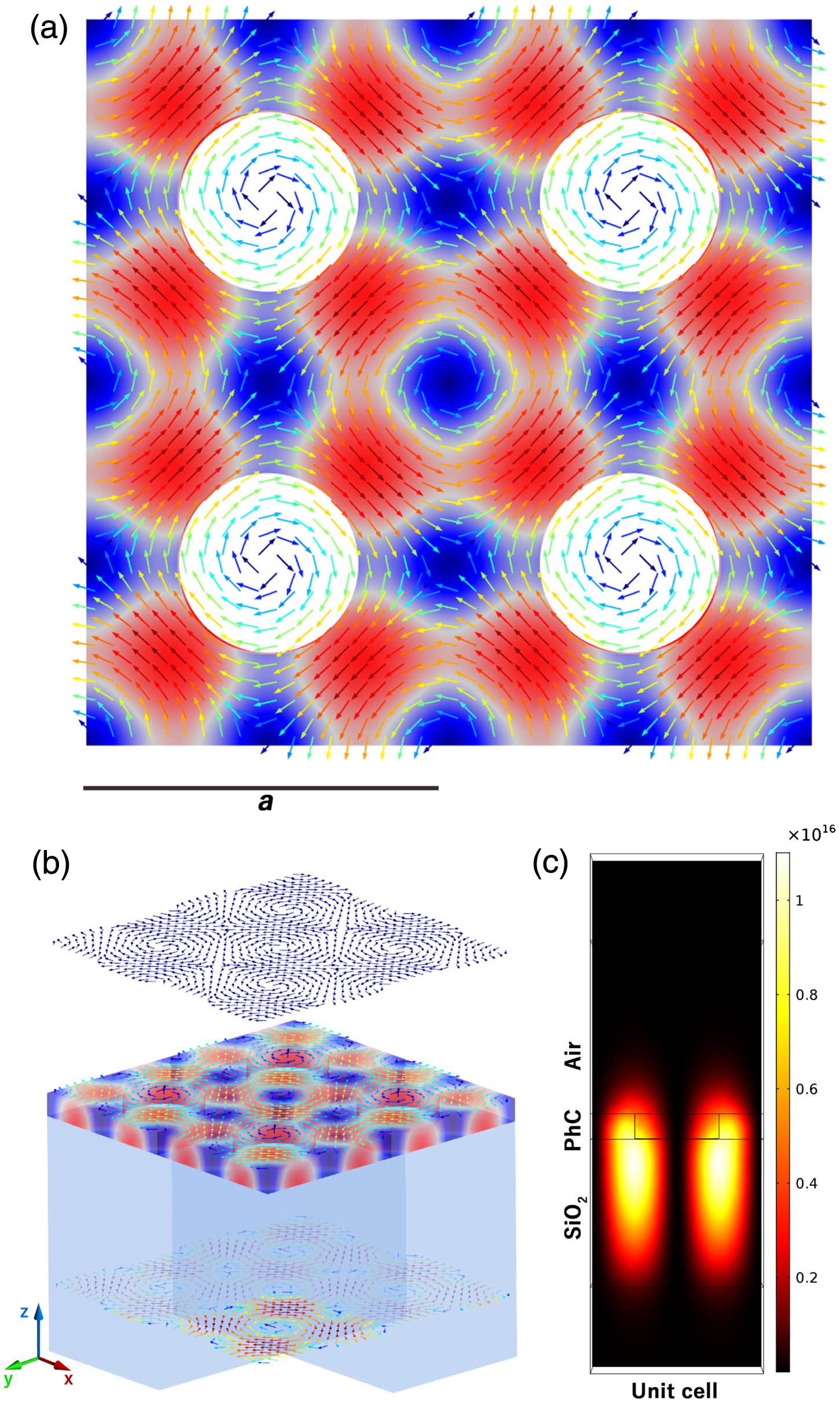
Fig. 1. (a) Calculated electric field in resonance condition at the BIC mode at the Γ a Si 3 N 4 / SiO 2 Si 3 N 4 / air Q
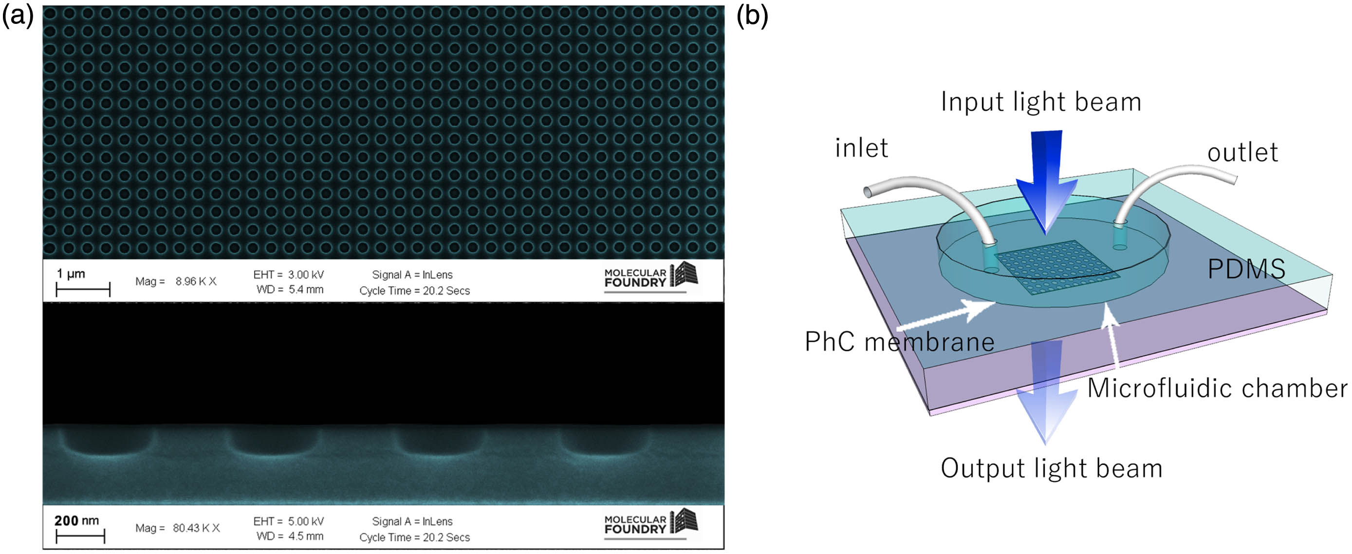
Fig. 2. (a) Scanning electron microscopy image of the PhCM sample. The design consists of air cylindrical holes arranged in a square lattice (a = 521 nm r = 130 nm h = 78 nm
Fig. 3. (a) Sketch of the experimental setup. SC source, supercontinuum source; P 1 P 2
Fig. 4. (a) BIC resonance excited in the PhC metasurfaces without the micro-chamber by a normally incident incoming beam. By fitting the measured spectrum (blue dots) with a Lorentzian line shape (purple curve), a linewidth and a quality factor as large as c / γ = 0.4 nm Q ≃ 2 × 10 3 S = 178 nm / RIU θ = 5 ° θ = 0 ° θ = − 5 °
Fig. 5. Reconstructed sensitivity curve in the visible range; the measurements demonstrated the scalability of the device, which reveals a bulk sensitivity S = 185 nm / RIU
Fig. 6. Cross-polarized transmission spectrum of the PhCM-based sensor prior (black curve) and post-functionalization with the self-assembling monolayer of BPT (red curve). When the BPT monolayer is assembled, a redshift at resonance wavelengths 1 and 2 occurred. A sensitivity of 6 nm of shift after the BPT monolayer formation was measured.

Set citation alerts for the article
Please enter your email address
© Copyright 2018-2021 | Chinese Laser Press. All Rights Reserved 沪ICP备15018463号-20