• High Power Laser Science and Engineering
  • Vol. 7, Issue 3, 03000e48 (2019)
Xue Dong1、2, Xingchen Pan1, Cheng Liu1、†, and Jianqiang Zhu1
Author Affiliations
  • 1Joint Laboratory on High-Power Laser and Physics, Shanghai Institute of Optics and Fine Mechanics, Chinese Academy of Sciences, Shanghai 201800, China
  • 2Center of Materials Science and Optoelectronics Engineering, University of Chinese Academy of Sciences, Beijing 100049, China
  • show less
    DOI: 10.1017/hpl.2019.26 Cite this Article Set citation alerts
    Xue Dong, Xingchen Pan, Cheng Liu, Jianqiang Zhu. An online diagnosis technique for simultaneous measurement of the fundamental, second and third harmonics in one snapshot[J]. High Power Laser Science and Engineering, 2019, 7(3): 03000e48 Copy Citation Text show less
    (a) Diagram of the CMI layout. The incident wave illuminates the phase modulator, which diffracts the observed light field into a speckle pattern. The speckle pattern and an iterative algorithm are used to retrieve the complex amplitude of the incident wave. (b) The designed three-step random phase plate. (c) One-dimensional diagram of (b).
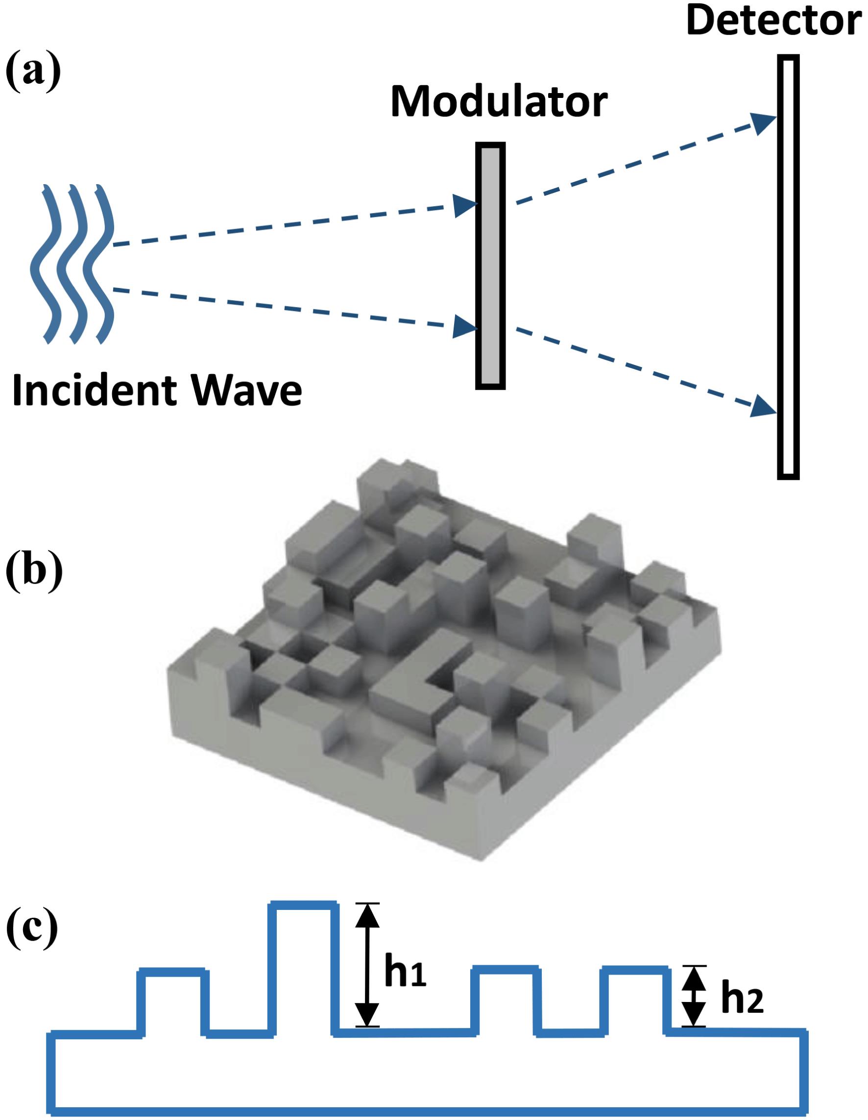
    Fig. 1. (a) Diagram of the CMI layout. The incident wave illuminates the phase modulator, which diffracts the observed light field into a speckle pattern. The speckle pattern and an iterative algorithm are used to retrieve the complex amplitude of the incident wave. (b) The designed three-step random phase plate. (c) One-dimensional diagram of (b).
    Flowchart of the reconstruction process.
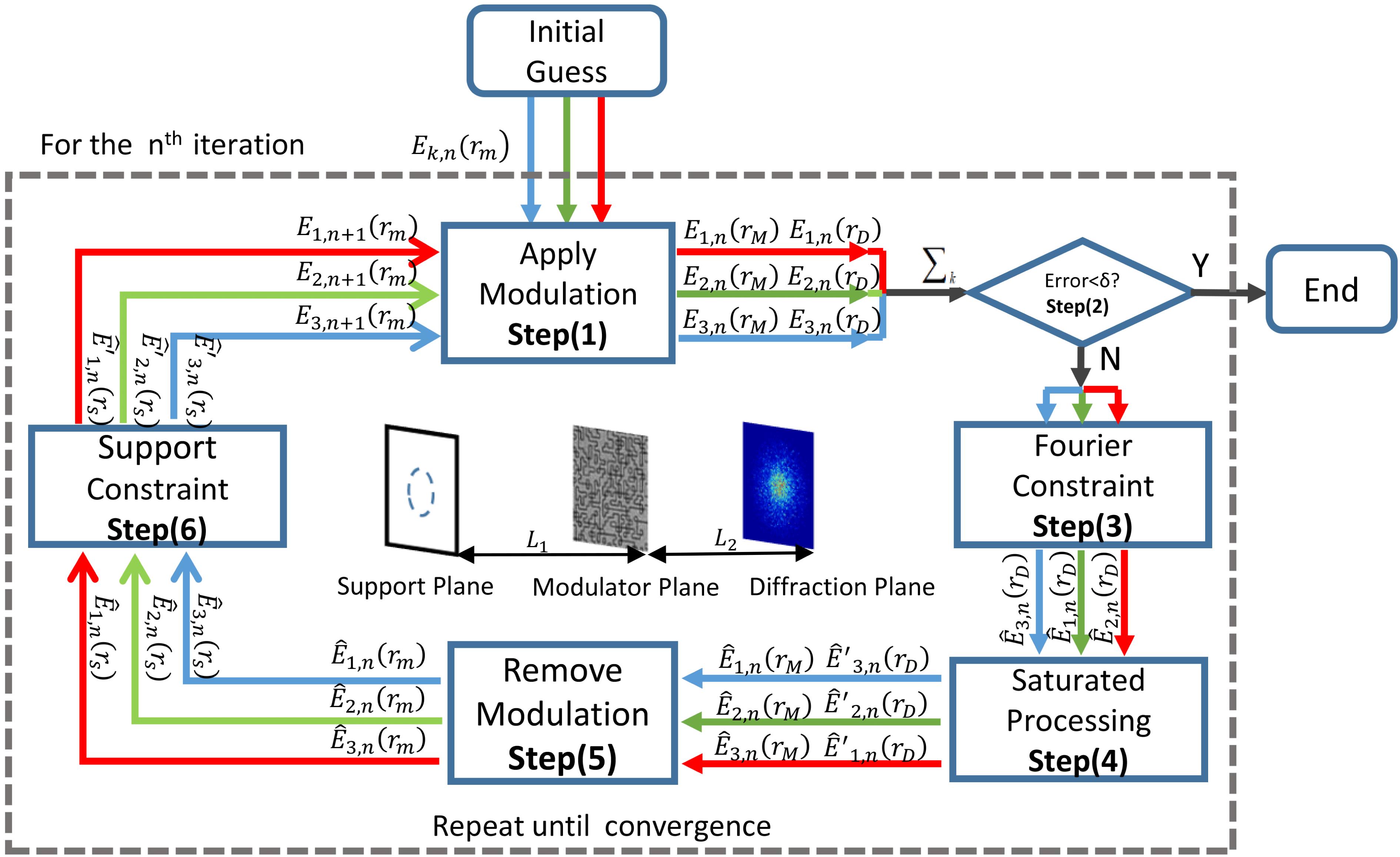
    Fig. 2. Flowchart of the reconstruction process.
    Beam path diagram of the simulation. The incident wave consists of frequencies $1\unicode[STIX]{x1D714}$, $2\unicode[STIX]{x1D714}$ and $3\unicode[STIX]{x1D714}$ simultaneously.
    Fig. 3. Beam path diagram of the simulation. The incident wave consists of frequencies $1\unicode[STIX]{x1D714}$, $2\unicode[STIX]{x1D714}$ and $3\unicode[STIX]{x1D714}$ simultaneously.
    (a)–(c) Amplitudes and (d)–(f) phases of these three illumination beams incident on the modulator plane for (a), (d) 351 nm, (b), (e) 526.5 nm and (c), (f) 1053 nm.
    Fig. 4. (a)–(c) Amplitudes and (d)–(f) phases of these three illumination beams incident on the modulator plane for (a), (d) 351 nm, (b), (e) 526.5 nm and (c), (f) 1053 nm.
    Phase delay of the modulator for (a) 351 nm, (b) 526.5 nm and (c) 1053 nm.
    Fig. 5. Phase delay of the modulator for (a) 351 nm, (b) 526.5 nm and (c) 1053 nm.
    Simulated diffraction patterns of (a) 351 nm, (b) 526.5 nm, (c) 1053 nm and (d) their summation, which is a hybrid diffraction pattern of the three wavelengths that provide simultaneous illumination. (e) Change in the corresponding reconstruction error for each wavelength throughout the iteration process.
    Fig. 6. Simulated diffraction patterns of (a) 351 nm, (b) 526.5 nm, (c) 1053 nm and (d) their summation, which is a hybrid diffraction pattern of the three wavelengths that provide simultaneous illumination. (e) Change in the corresponding reconstruction error for each wavelength throughout the iteration process.
    Three illuminations incident on the modulator plane for (a) 351 nm, (b) 526.5 nm, (c) 1053 nm with different lens aberrations.
    Fig. 7. Three illuminations incident on the modulator plane for (a) 351 nm, (b) 526.5 nm, (c) 1053 nm with different lens aberrations.
    (A) Beam path diagram of the second simulation. The wavefronts behind the ‘SG’ phase plate for (a) 351 nm, (b) 526.5 nm and (c) 1053 nm. (d)–(f) plot their phase delay profile along the white line in (a)–(c), respectively. (g)–(i) display the amplitude of the three incident beams on the modulator plane.
    Fig. 8. (A) Beam path diagram of the second simulation. The wavefronts behind the ‘SG’ phase plate for (a) 351 nm, (b) 526.5 nm and (c) 1053 nm. (d)–(f) plot their phase delay profile along the white line in (a)–(c), respectively. (g)–(i) display the amplitude of the three incident beams on the modulator plane.
    (a)–(c) Reconstructed modulus and (d)–(f) phase on the modulator plane for 351 nm, 526.5 nm and 1053 nm, respectively. (g)–(i) show the wavefronts behind the ‘SG’ phase plate. (j)–(l) plot the reconstructed phase delay profile along the white line in (g)–(i), respectively.
    Fig. 9. (a)–(c) Reconstructed modulus and (d)–(f) phase on the modulator plane for 351 nm, 526.5 nm and 1053 nm, respectively. (g)–(i) show the wavefronts behind the ‘SG’ phase plate. (j)–(l) plot the reconstructed phase delay profile along the white line in (g)–(i), respectively.
    Experimental setup for measuring the fundamental, second and third harmonics in one snapshot.
    Fig. 10. Experimental setup for measuring the fundamental, second and third harmonics in one snapshot.
    (a)–(c) Reconstructed amplitude and (d)–(f) phase of the random phase plate for 351 nm, 526.5 nm and 1053 nm, respectively, using ptychography.
    Fig. 11. (a)–(c) Reconstructed amplitude and (d)–(f) phase of the random phase plate for 351 nm, 526.5 nm and 1053 nm, respectively, using ptychography.
    Recorded diffraction pattern (A) and reconstructed results of the three harmonics of the random phase plate with our proposed method. (a1)–(c1) Amplitude and (a2)–(c2) phase of 351 nm, 526.5 nm and 1053 nm, respectively. Wavefronts before the convergent lens for (a3) 351 nm, (b3) 526.5 nm and (c3) 1053 nm.
    Fig. 12. Recorded diffraction pattern (A) and reconstructed results of the three harmonics of the random phase plate with our proposed method. (a1)–(c1) Amplitude and (a2)–(c2) phase of 351 nm, 526.5 nm and 1053 nm, respectively. Wavefronts before the convergent lens for (a3) 351 nm, (b3) 526.5 nm and (c3) 1053 nm.
    Single-wavelength CMI results. (a1)–(c1) Recorded diffraction pattern associated with each wavelength. (a2)–(c2) Amplitude and (a3)–(c3) phase for 351 nm, 526.5 nm and 1053 nm, respectively. Wavefronts before the convergent lens for (a4) 351 nm, (b4) 526.5 nm and (c4) 1053 nm.
    Fig. 13. Single-wavelength CMI results. (a1)–(c1) Recorded diffraction pattern associated with each wavelength. (a2)–(c2) Amplitude and (a3)–(c3) phase for 351 nm, 526.5 nm and 1053 nm, respectively. Wavefronts before the convergent lens for (a4) 351 nm, (b4) 526.5 nm and (c4) 1053 nm.
    Evolution of the error curve versus iterations. (a) Results of the three-wavelength CMI reconstruction error for 351 nm (blue), 526.5 nm (green) and 1053 nm (red). (b) Results for the single-wavelength CMI error using the same procedure as (a).
    Fig. 14. Evolution of the error curve versus iterations. (a) Results of the three-wavelength CMI reconstruction error for 351 nm (blue), 526.5 nm (green) and 1053 nm (red). (b) Results for the single-wavelength CMI error using the same procedure as (a).
    Reconstructed results for a step phase plate: (a) 351 nm, (b) 526.5 nm, (c) 1053 nm. (d)–(f) plot the red solid line in (a)–(c), respectively.
    Fig. 15. Reconstructed results for a step phase plate: (a) 351 nm, (b) 526.5 nm, (c) 1053 nm. (d)–(f) plot the red solid line in (a)–(c), respectively.
    Xue Dong, Xingchen Pan, Cheng Liu, Jianqiang Zhu. An online diagnosis technique for simultaneous measurement of the fundamental, second and third harmonics in one snapshot[J]. High Power Laser Science and Engineering, 2019, 7(3): 03000e48
    Download Citation