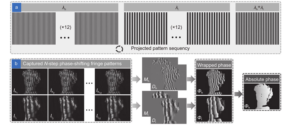
Fig. 1. The process of generating training data. (a) The projection mode includes dual-frequency 12-step phase-shifting fringe projection patterns and dual-frequency composite fringe pattern. (b) A set of captured images and the corresponding labels contain numerator term, denominator term, and absolute phase map.

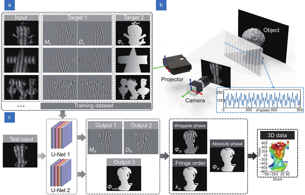
Fig. 2. Flowchart of our proposed approach. (a) Part of network training data sets. (b) Hardware system and the cross-section intensity distribution of the designed composite fringe pattern. (c) Test data and prediction results obtained by the training model.

Fig. 3. The U-Net network architecture.

Fig. 4. Comparison between one U-Net network and two U-Net networks (the proposed method). (a, d, g, j) The raw composite fringe images from four different measurement scenes. (b, e, h, k) The absolute phase result error between deep-learning-predicted value and the ground-truth value by using one U-Net network. (c, f, i, l) The absolute phase result error between deep-learning-predicted value and the ground-truth value by using two U-Net networks.

Fig. 5. Part of input training datasets. The surface shapes contain single complex surface, geometric surface and discontinuous surface, and the materials include plaster, plastic, and paper.

Fig. 6. Four sets of network test inputs in static scenarios (a–d) and their corresponding spectral cross-sectional intensity distributions (e–h).

Fig. 7. The prediction results of our proposed method (DCFPP) in four static scenarios. (a, e, i, m) The numerator Mdl results. (b, f, j, n) The denominator Ddl results. (c, g, k, o) The wrapped phase Φdl results. (d, h, l, p) The high-quality absolute phase maps Φdl.

Fig. 8. Phase error comparison results of traditional dual-frequency composite FT method and the proposed DCFPP method. (a, e, i, m) The wrapped phase error calculated by traditional method. (b, f, j, n) The wrapped phase error predicted by the DCFPP. (c, g, k, o) The absolute phase error of traditional method. (d, h, l, p) The absolute phase error of the DCFPP.

Fig. 9. 3D reconstruction results of end-to-end network, the proposed DCFPP and 12-step PS with number-theoretic method in four measurement scenes. (a, d, g, j) 3D reconstruction results of the end-to-end network. (b, e, h, k) 3D reconstruction results of DCFPP. (c, f, i, l) 3D reconstruction results obtained by 12-step PS with number-theoretic method (ground-truth).

Fig. 10. Measurement results of a dynamic scene. (a, c) The captured composite fringe images at two different moments. (b, d) The corresponding 3D results reconstructed by DCFPP. (Multimedia view: see Supplementary information Visualization 1 for the whole measurement process of the rotating plaster statue)

Fig. 11. Precision analysis of standard ceramic plate and a standard ceramic sphere. (a, d) 3D reconstruction results by DCFPP. (b, e) Error distribution. (c, f) RMS error.

Table 1. MAE of wrapped phase and absolute phase of the traditional dual-frequency composite FT method and the proposed DCFPP method (noted that the “FT method” mentioned in the table refers to the traditional dual-frequency composite FT method).