
Haoran Gu, Zhengqiang Li, Weizhen Hou, Zhenhai Liu, Lili Qie, Yinna Li, Yang Zheng, Zheng Shi, Hua Xu, Jin Hong, Jinji Ma, Zhenting Chen. Information Content Analysis on Passive Remote Sensing Imaging Retrieval of Aerosol Layer Height Based on Spaceborne Polarization Crossfire[J]. Acta Optica Sinica, 2023, 43(6): 0601003
- Acta Optica Sinica
- Vol. 43, Issue 6, 0601003 (2023)
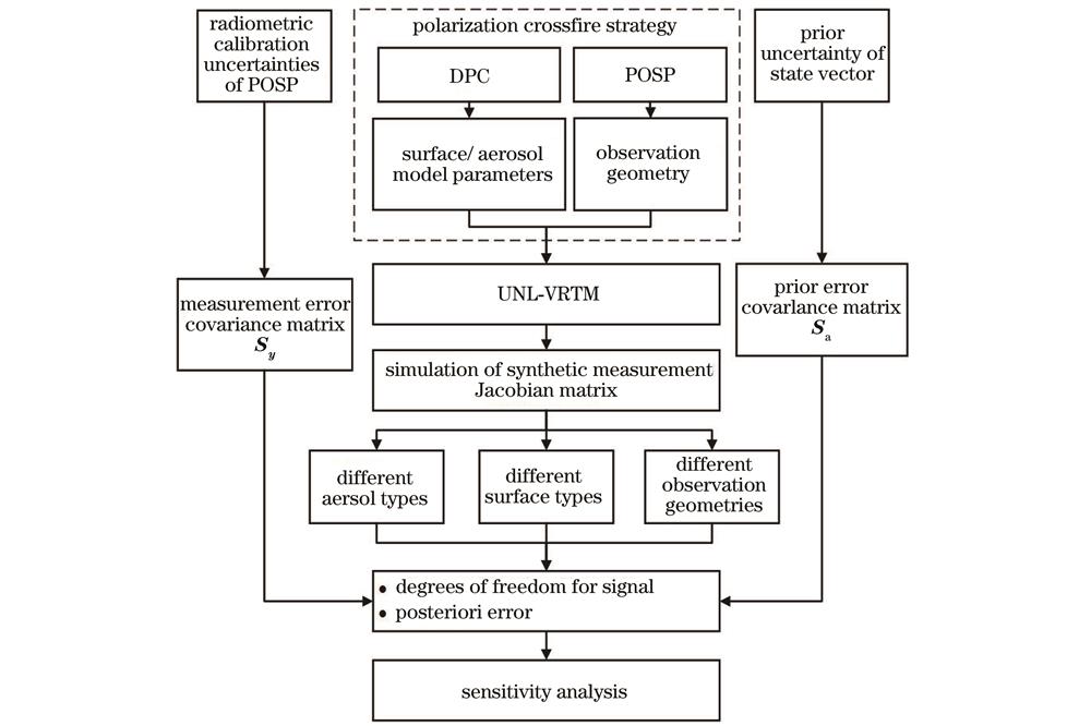
Fig. 1. Flowchart of information content analysis
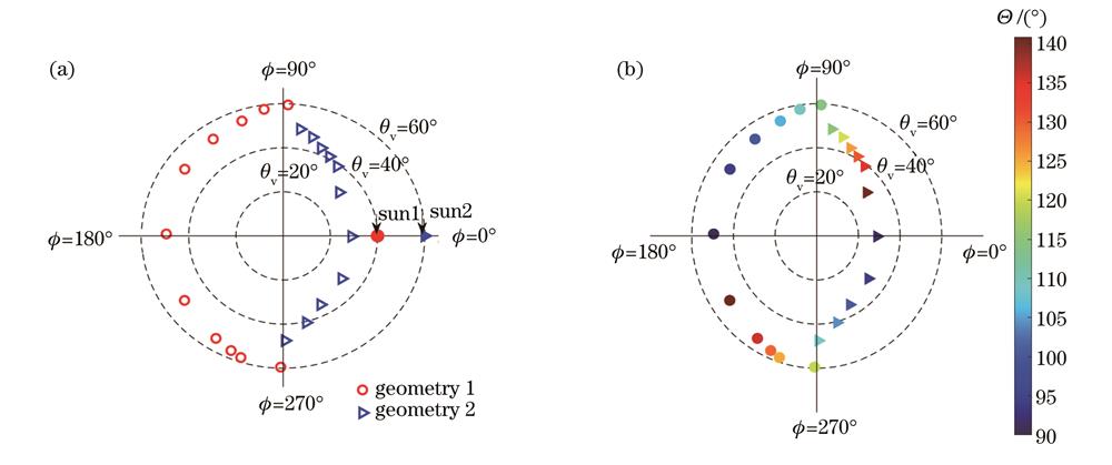
Fig. 2. PSOP observation geometry used in research. (a) Observation geometry; (b) scattering angle distribution
Fig. 3. Aerosol volume size distribution
Fig. 4. Scattering phase function and polarized scattering phase function varying with scattering angle. (a)(b) Scattering phase function; (c)(d) polarized scattering phase function
Fig. 5. Surface simulation results varying with observation geometry angle. (a) BRDF; (b) BPDF
Fig. 6. Simulation result varying with observation geometry angle. (a) Apparent reflectivity ; (b) apparent polarized reflectivity
Fig. 7. Jacobian result varying with observation geometry angle. (a)
Fig. 8. Jacobian result of vegetation surface intensity observation varying with H under different observation geometries. (a) Fine-dominated AOD of 0.8; (b) coarse-dominated AOD of 0.8; (c) fine-dominated AOD of 0.2; (d) coarse-dominated AOD of 0.2
Fig. 9. Jacobi simulation results under different aerosol and vegetation surface conditions. (a) (c) Different aerosol conditions; (b)(d) different surface conditions
Fig. 10. Analysis of information content results under different surface conditions. (a) Vegetation; (b) bare soil
Fig. 11. ALH information under different scenarios. (a) Fine-dominated; (b) coarse-dominated
Fig. 12. Posterior error varying with aerosol model parameters at 380 nm band. (a)(b) Posterior error; (c)(d) reduction value of posterior error
Fig. 13. Effect of adding 380 nm wave band polarization measurement on posterior error. (a)(b) Adding 380 nm wave band pure intensity measurement; (c)(d) adding 380 nm wave band intensity and polarization measurements; (e)(f) difference of posterior error reduction between two observation schemes
Fig. 14. Effect of adding 410 nm measurement on posterior error. (a)(b) Adding 410 nm band intensity measurement; (c)(d) adding 410 nm band intensity and polarization measurements
|
Table 1. Basic parameters of sensors
|
Table 2. Aerosol model parameters
|
Table 3. Surface model parameters
|
Table 4. POSP observable correlation in 380 nm and 410 nm
|
Table 5. Numerical simulation schemes
|
Table 6. DFS of H at A-I and AV-IP schemes

Set citation alerts for the article
Please enter your email address
© Copyright 2018-2021 | Chinese Laser Press. All Rights Reserved 沪ICP备15018463号-20