• Laser & Optoelectronics Progress
  • Vol. 58, Issue 12, 1212004 (2021)
Jun Gu*
Author Affiliations
  • College of Information Engineering, Jiangsu Open University, Nanjing, Jiangsu 210019, China
  • show less
    DOI: 10.3788/LOP202158.1212004 Cite this Article Set citation alerts
    Jun Gu. Strain Field Calculation by 3D Digital Image Correlation Method Based on Subset Projection and Savitzky-Golay Filter[J]. Laser & Optoelectronics Progress, 2021, 58(12): 1212004 Copy Citation Text show less
    Principle diagram of two-dimensional DIC
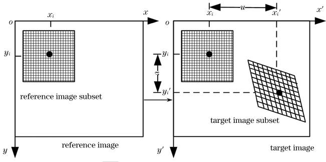
    Fig. 1. Principle diagram of two-dimensional DIC
    Flow chart of DIC calculation. (a) 2D; (b) 3D
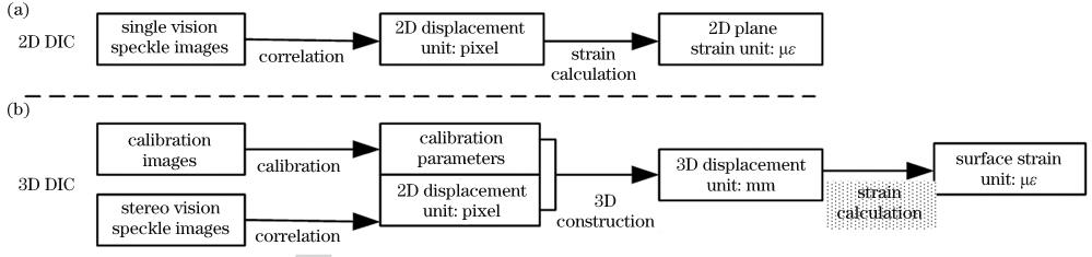
    Fig. 2. Flow chart of DIC calculation. (a) 2D; (b) 3D
    Schematic of tangential plane projection method
    Fig. 3. Schematic of tangential plane projection method
    Schematic of displacement field in strain calculation subset. (a) u; (b) v
    Fig. 4. Schematic of displacement field in strain calculation subset. (a) u; (b) v
    Simulated morphology with homogeneous deformation (no noise)
    Fig. 5. Simulated morphology with homogeneous deformation (no noise)
    Simulated strain fields with homogeneous deformation and error (M=5 and no noise). (a) Positive strain along x direction; (b) positive strain along y direction; (c) tangential strain; (d) strain field error along x direction
    Fig. 6. Simulated strain fields with homogeneous deformation and error (M=5 and no noise). (a) Positive strain along x direction; (b) positive strain along y direction; (c) tangential strain; (d) strain field error along x direction
    Simulated morphology with inhomogeneous deformation (no noise)
    Fig. 7. Simulated morphology with inhomogeneous deformation (no noise)
    Simulated strain fields with inhomogeneous deformation and error (M=5 and no noise). (a) Positive strain along x direction; (b) positive strain along y direction; (c) tangential strain; (d) strain field error along x direction
    Fig. 8. Simulated strain fields with inhomogeneous deformation and error (M=5 and no noise). (a) Positive strain along x direction; (b) positive strain along y direction; (c) tangential strain; (d) strain field error along x direction
    Simulated strain fields with homogeneous deformation and error (M=5,σx,y=0.001 mm,σz=0.004 mm). (a) Positive strain along x direction; (b) positive strain along y direction; (c) tangential strain; (d) strain field error along x direction
    Fig. 9. Simulated strain fields with homogeneous deformation and error (M=5,σx,y=0.001 mm,σz=0.004 mm). (a) Positive strain along x direction; (b) positive strain along y direction; (c) tangential strain; (d) strain field error along x direction
    Simulated strain fields with homogeneous deformation and error (M=10,σx,y=0.001 mm,σz=0.004 mm). (a) Positive strain along x direction; (b) positive strain along y direction; (c) tangential strain; (d) strain field error along x direction
    Fig. 10. Simulated strain fields with homogeneous deformation and error (M=10,σx,y=0.001 mm,σz=0.004 mm). (a) Positive strain along x direction; (b) positive strain along y direction; (c) tangential strain; (d) strain field error along x direction
    Simulated strain fields with inhomogeneous deformation and error (M=5,σx,y=0.001 mm,σz=0.004 mm). (a) Positive strain along x direction; (b) positive strain along y direction; (c) tangential strain; (d) strain field error along x direction
    Fig. 11. Simulated strain fields with inhomogeneous deformation and error (M=5,σx,y=0.001 mm,σz=0.004 mm). (a) Positive strain along x direction; (b) positive strain along y direction; (c) tangential strain; (d) strain field error along x direction
    Simulated strain fields with inhomogeneous deformation and error (M=10,σx,y=0.001 mm,σz=0.004 mm). (a) Positive strain along x direction; (b) positive strain along y direction; (c) tangential strain; (d) strain field error along x direction
    Fig. 12. Simulated strain fields with inhomogeneous deformation and error (M=10,σx,y=0.001 mm,σz=0.004 mm). (a) Positive strain along x direction; (b) positive strain along y direction; (c) tangential strain; (d) strain field error along x direction
    Schematic of experimental system
    Fig. 13. Schematic of experimental system
    Strain field distributions of thin plate. (a) εxx; (b) εyy;(c)γxy
    Fig. 14. Strain field distributions of thin plate. (a) εxx; (b) εyy;(c)γxy
    ConditionDeformationFilter sizeeεεσεε
    No noiseHomogeneousM=52.22×10-102.22×10⁻¹⁰
    InhomogeneousM=52.20×10-102.74×10⁻¹⁰
    Gaussian noise with σx,y=0.001 mm andσz=0.004 mmHomogeneousM=524.1730.11
    HomogeneousM=106.518.36
    InhomogeneousM=523.1529.28
    InhomogeneousM=106.889.36
    Table 1. Statistics of strain field errors along x direction
    Calibration parameterUnitValue
    k1mm-21.56×10⁻¹
    k2mm-44.28×10⁻¹
    p1mm-1-1.56×10⁻³
    p2mm-1-3.17×10⁻⁴
    Rx°3.06×10⁻¹
    Ry°2.96×10
    Rz°1.01×10⁻¹
    Txmm-2.78×10²
    Tymm2.49×10-1
    Tzmm7.98×10
    Table 2. Main calibration parameters
    Jun Gu. Strain Field Calculation by 3D Digital Image Correlation Method Based on Subset Projection and Savitzky-Golay Filter[J]. Laser & Optoelectronics Progress, 2021, 58(12): 1212004
    Download Citation