• Photonics Research
  • Vol. 11, Issue 2, 212 (2023)
Lei Yuan1, Qiang Song2, Hecong Liu1, Kevin Heggarty3, and Weiwei Cai1、*
Author Affiliations
  • 1Key Laboratory for Power Machinery and Engineering of the Ministry of Education, School of Mechanical Engineering, Shanghai Jiao Tong University, Shanghai 200240, China
  • 2Lochn Optics, Shenzhen 518200, China
  • 3Optics Department, IMT-Atlantique, Technopole Brest-Iroise, CS 83818, 29285 Brest, France
  • show less
    DOI: 10.1364/PRJ.472072 Cite this Article Set citation alerts
    Lei Yuan, Qiang Song, Hecong Liu, Kevin Heggarty, Weiwei Cai. Super-resolution computed tomography imaging spectrometry[J]. Photonics Research, 2023, 11(2): 212 Copy Citation Text show less
    Schematic of the SRCTIS system. The input image is split into two by a beam splitter and collected by an RGB camera and a conventional CTIS system, respectively. In the CTIS branch, after collimation, the input image is diffracted by the DOE and received by a gray camera.
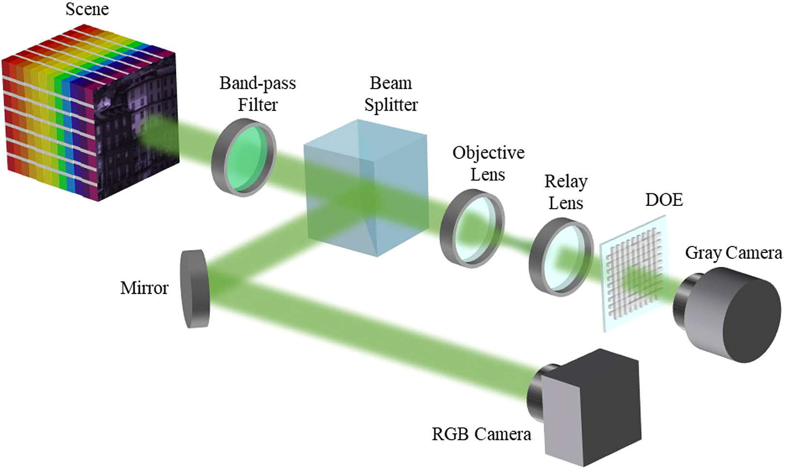
    Fig. 1. Schematic of the SRCTIS system. The input image is split into two by a beam splitter and collected by an RGB camera and a conventional CTIS system, respectively. In the CTIS branch, after collimation, the input image is diffracted by the DOE and received by a gray camera.
    Principle of SRCTIS for reconstruction of a data cube with both high spatial and spectral resolutions. First, the CTIS reconstruction and an RGB image are obtained separately; then the CTIS multispectral pixels and the RGB image pixels are aligned by position calibration; and finally, a spectral propagation algorithm is used to fuse the two images.
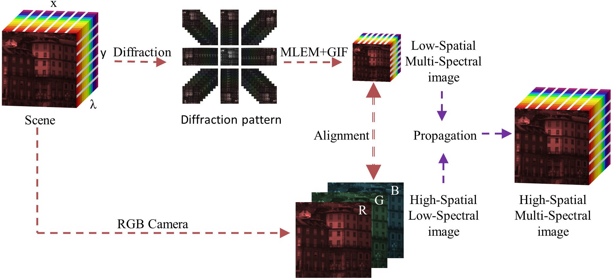
    Fig. 2. Principle of SRCTIS for reconstruction of a data cube with both high spatial and spectral resolutions. First, the CTIS reconstruction and an RGB image are obtained separately; then the CTIS multispectral pixels and the RGB image pixels are aligned by position calibration; and finally, a spectral propagation algorithm is used to fuse the two images.
    Flowchart of the MLEM algorithm with GIF. After each MLEM iteration, GIF is applied to suppress the reconstruction artifacts.
    Fig. 3. Flowchart of the MLEM algorithm with GIF. After each MLEM iteration, GIF is applied to suppress the reconstruction artifacts.
    (a) Calibrated RGB response curves; (b) projection of the CTIS multispectral pixels on the RGB image. The yellow pixels have unknown multispectral but known RGB details, and the blue pixels have both known RGB and multispectral details.
    Fig. 4. (a) Calibrated RGB response curves; (b) projection of the CTIS multispectral pixels on the RGB image. The yellow pixels have unknown multispectral but known RGB details, and the blue pixels have both known RGB and multispectral details.
    (a) Ground truth and the corresponding reconstructions of different scenes (denoted in sequence from left to right as “flowers,” “oil painting,” “cloth,” and “toys”) from MLEM and MLEM_GIF with the quality metrics PSNR/SSIM/SAM labeled at the bottom of each reconstructed image; (b) the relationships between the noise level and the different reconstruction quality metrics.
    Fig. 5. (a) Ground truth and the corresponding reconstructions of different scenes (denoted in sequence from left to right as “flowers,” “oil painting,” “cloth,” and “toys”) from MLEM and MLEM_GIF with the quality metrics PSNR/SSIM/SAM labeled at the bottom of each reconstructed image; (b) the relationships between the noise level and the different reconstruction quality metrics.
    Comparison of the spatial details of different scenes (denoted in sequence from top to bottom as “lilies,” “ruined house,” and “roof”) reconstructed from MLEM, MLEM_GIF, and SRCTIS. The enlarged images in the upper left corner, respectively, represent randomly selected local areas in the corresponding scene.
    Fig. 6. Comparison of the spatial details of different scenes (denoted in sequence from top to bottom as “lilies,” “ruined house,” and “roof”) reconstructed from MLEM, MLEM_GIF, and SRCTIS. The enlarged images in the upper left corner, respectively, represent randomly selected local areas in the corresponding scene.
    (a) Spectra for randomly selected points (marked A, B, and C) in Fig. 6 from the ground truth, MLEM, MLEM_GIF, and SRCTIS reconstructions, respectively; (b) quantitative image quality metrics and computational time for reconstructing 10 scenes with a discretization of 200×200×57 under 25-dB noise.
    Fig. 7. (a) Spectra for randomly selected points (marked A, B, and C) in Fig. 6 from the ground truth, MLEM, MLEM_GIF, and SRCTIS reconstructions, respectively; (b) quantitative image quality metrics and computational time for reconstructing 10 scenes with a discretization of 200×200×57 under 25-dB noise.
    Quantitative comparison of different algorithms in terms of spatial and spectral resolutions. Panel (a) presents the modulation transfer functions corresponding to CTIS, SRCTIS, CTIS with the nearest-neighbor interpolation, and the RGB camera; panel (b) presents the reconstructed spectrum of CTIS where the reference spectrum contains two peaks at 495 nm and 505 nm, respectively; panel (c) presents the reconstructed spectrum of SRCTIS where the reference spectrum contains two peaks at 493 nm and 505 nm, respectively.
    Fig. 8. Quantitative comparison of different algorithms in terms of spatial and spectral resolutions. Panel (a) presents the modulation transfer functions corresponding to CTIS, SRCTIS, CTIS with the nearest-neighbor interpolation, and the RGB camera; panel (b) presents the reconstructed spectrum of CTIS where the reference spectrum contains two peaks at 495 nm and 505 nm, respectively; panel (c) presents the reconstructed spectrum of SRCTIS where the reference spectrum contains two peaks at 493 nm and 505 nm, respectively.
    (a) Experimental reconstructions of different scenes (denoted in sequence from top to bottom as “hills,” “sailboat,” “landscape painting,” and “blueberries”) from MLEM, MLEM_GIF, and SRCTIS, respectively; (b) reconstruction results of the hills scene at different wavelengths under SRCTIS; (c) spectra of randomly selected points (marked A, B, C, and D) from different scenes shown in panel (a).
    Fig. 9. (a) Experimental reconstructions of different scenes (denoted in sequence from top to bottom as “hills,” “sailboat,” “landscape painting,” and “blueberries”) from MLEM, MLEM_GIF, and SRCTIS, respectively; (b) reconstruction results of the hills scene at different wavelengths under SRCTIS; (c) spectra of randomly selected points (marked A, B, C, and D) from different scenes shown in panel (a).
    Lei Yuan, Qiang Song, Hecong Liu, Kevin Heggarty, Weiwei Cai. Super-resolution computed tomography imaging spectrometry[J]. Photonics Research, 2023, 11(2): 212
    Download Citation