Researching | Terahertz spin dynamics in rare-earth orthoferrites

Journals >Photonics Insights >Volume 1 >Issue 2 >Page R05 > Article

Photonics Insights
Vol. 1, Issue 2, R05 (2022)

Terahertz spin dynamics in rare-earth orthoferrites | Story Video , On the Cover

Xinwei Li^1、2, Dasom Kim^2、3, Yincheng Liu¹, and Junichiro Kono^{2、4、5、*}

Author Affiliations

¹Department of Physics, California Institute of Technology, Pasadena, USA

²Department of Electrical and Computer Engineering, Rice University, Houston, USA

³Applied Physics Graduate Program, Smalley-Curl Institute, Rice University, Houston, USA

⁴Department of Physics and Astronomy, Rice University, Houston, USA

⁵Department of Materials Science and NanoEngineering, Rice University, Houston, USA

show less

DOI: 10.3788/PI.2022.R05 Cite this Article Set citation alerts

Xinwei Li, Dasom Kim, Yincheng Liu, Junichiro Kono. Terahertz spin dynamics in rare-earth orthoferrites[J]. Photonics Insights, 2022, 1(2): R05 Copy Citation Text

show less

Overview of current scientific and technological interests related to spin dynamics in solid-state materials. Four topics arranged as smaller triangular elements are covered in this review, which are key elements for achieving the three grander goals (three sides of the larger triangle).

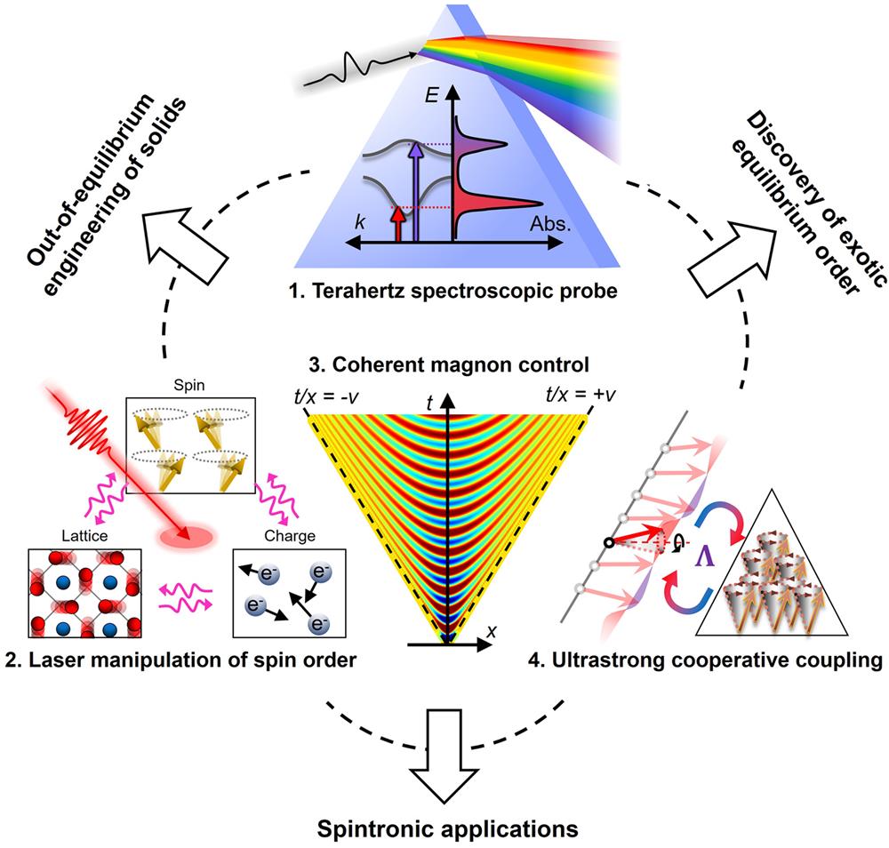
Fig. 1. Overview of current scientific and technological interests related to spin dynamics in solid-state materials. Four topics arranged as smaller triangular elements are covered in this review, which are key elements for achieving the three grander goals (three sides of the larger triangle).

Download full size | View in the Article

“Phase space” for review articles in spintronics, spanned by the horizontal axis of materials and vertical axis of novel physical phenomena. The current review represents a vertical cut in the phase space.

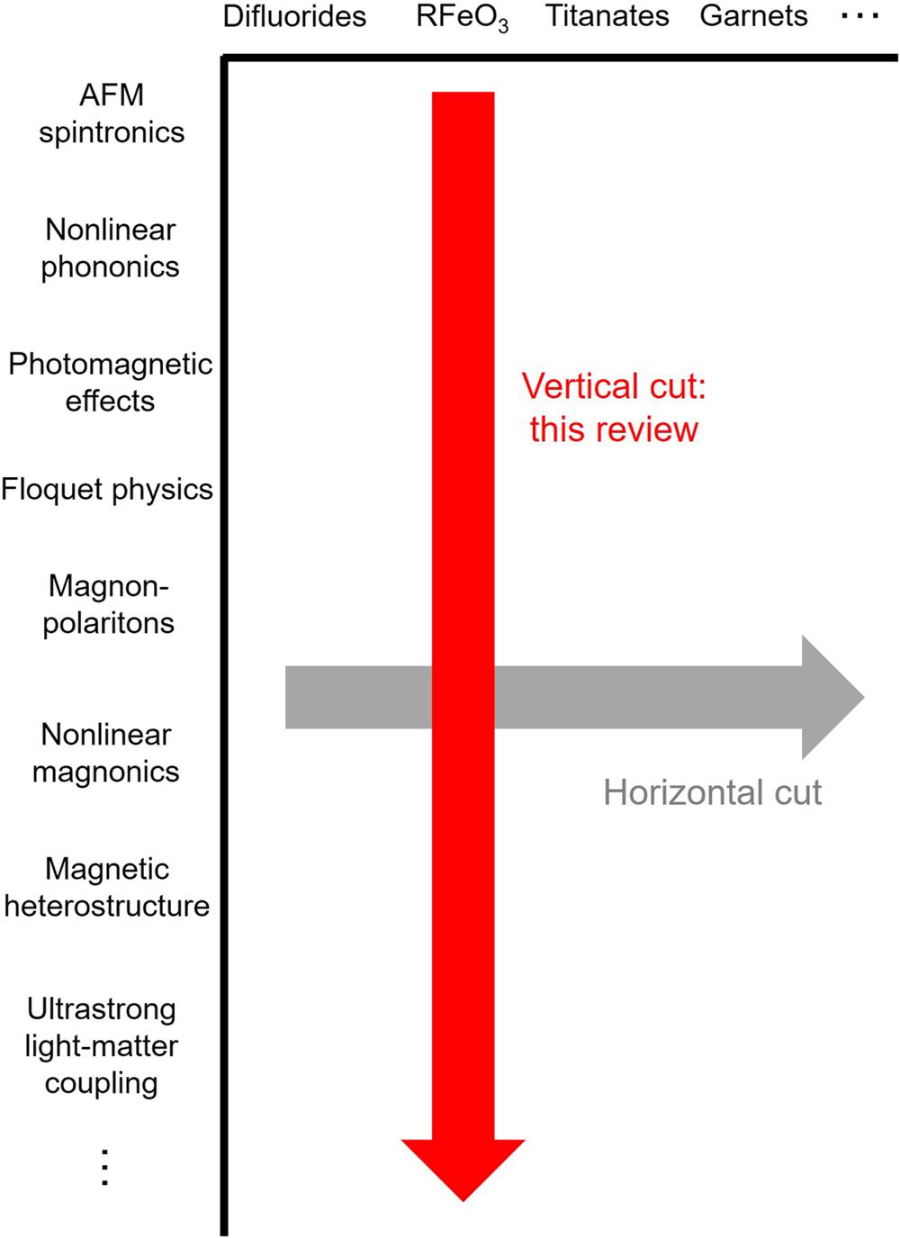
Fig. 2. “Phase space” for review articles in spintronics, spanned by the horizontal axis of materials and vertical axis of novel physical phenomena. The current review represents a vertical cut in the phase space.

Download full size | View in the Article

Fig. 3. Temperature-dependent magnetic phase diagrams for all members of the

{RFeO}_{3}

class^[79], except for

R = Pm

, for which no data are available due to its radioactivity. SRT, spin reorientation transition. Reproduced with permission from Ref. [79].

Download full size | View in the Article

Fig. 4. Basic physical properties of

{RFeO}_{3}

crystals. (a) Temperature-dependent magnetization of

{LuFeO}_{3}

,

{ErFeO}_{3}

, and

{DyFeO}_{3}

along the

z

axis and

x

axis^[75]. (b) Optical absorption spectrum of

{ErFeO}_{3}

^[94]. (c) Spin-wave dispersion mapped by inelastic neutron scattering^[95]. (d) Spin oscillations in quasi-FM and quasi-AFM modes^[96]. Each spin evolves in the sequence of

1 \to 2 \to 3 \to 4 \to 1 \dots

. Spins are synchronized by the number label. Reproduced with permission from Refs. [75,94

–

96].

Download full size | View in the Article

Fig. 5. Observation of (a) the inverse Faraday effect^[118] and (b) the inverse Cotton–Mouton effect^[119] in

{DyFeO}_{3}

. The oscillation phases of magnons excited by these photomagnetic effects depend on the polarization of the pump light. (c) Magnon excitation by the two photomagnetic effects can be described by the framework of impulsive stimulated Raman scattering^[57]. Reproduced with permission from Refs. [57,118,119].

Download full size | View in the Article

Fig. 6. Path of solving for the full dynamics of photomagnetic pump, magneto-optical probe experiments on

{RFeO}_{3}

, summarized from the procedure adopted in Ref. [119].

Download full size | View in the Article

Fig. 7. THz time-domain techniques. (a) Layout of a THz time-domain spectroscopy setup configured in a transmission geometry. (b) Zoom-in view of the polarization-sensitive differential detection setup^[36]. (c) Layout of a THz emission spectroscopy setup. (d) Function of a reflective echelon used in a single-shot THz spectrometer^[138]. (e) Pulse-front-tilt technique for generating intense THz radiation in

{LiNbO}_{3}

^[38]. BS, beam splitter; QWP, quarter-wave plate; WP, Wollaston prism; BD, balanced detector. (b), (d), (e) Reproduced with permission from Refs. [36,38,138].

Download full size | View in the Article

Fig. 8. Six measurement configurations, along with the magnon polarization selection rule in the

Γ_{4}

and

Γ_{2}

phases. The magnetic field component of the THz pulse

H_{THz}

is polarized along a line whose color indicates the magnon mode that can be excited. The THz propagation direction is perpendicular to the disk containing the line. Reproduced with permission from Ref. [169].

Download full size | View in the Article

Fig. 9. Temperature-dependent SRT probed by THz spectroscopy^{[170–172" target="_self" style="display: inline;">–172]}. (a) Switching of the polarization selection rule. (b) Switching of the polarization trajectory of magnon emission. (c) Experimental verification of (b). (d) Continuous spectral weight transfer between two measurement configurations of the quasi-AFM mode amplitude. (e), (f) Quantifying the rotation angle during the SRT from quasi-AFM to quasi-FM mode spectral weight transfer in

z

-cut

{Dy}_{0.7} {Er}_{0.3} {FeO}_{3}

. Inset to (f): calculated free-energy landscape at various temperatures (red to blue: low to high temperatures). Reproduced with permission from Refs. [170

172" target="_self" style="display: inline;">–172].

Download full size | View in the Article

Fig. 10. Magnetic-field-induced

Γ_{4} \to Γ_{2}

SRT probed by THz spectroscopy^[174,175]. (a) Observation of switching of the polarization selection rule in

{NdFeO}_{3}

. (b) Field-dependent absorption spectra in

{YFeO}_{3}

. (c) Calculated quasi-FM and quasi-AFM frequencies versus magnetic field, to compare with (b). Reproduced with permission from Refs. [174,175].

Download full size | View in the Article

Fig. 11. CFTs of

{Tm}^{3 +}

ions in

{TmFeO}_{3}

^[179]. (a) Absorption coefficient mapped as a function of frequency and temperature. Red circles: quasi-AFM mode. Blue squares: quasi-FM mode. (b) Constant-temperature cut of absorption coefficient at 60 K for three different measurement configurations. (c) Energy-level diagram explaining the THz transitions. Reproduced with permission from Ref. [179].

Download full size | View in the Article

Fig. 12. CFTs of

{Er}^{3 +}

in

{ErFeO}_{3}

^[169]. (a) Energy-level scheme of

{Er}^{3 +}

. Levels shown in red lines are involved in the transitions observed in experiments. (b) Two-sublattice model. Magneto-THz absorption spectra from measurements in (c) configuration 1, (d) configuration 4, and (e) configuration 6. (f)–(h) Energy-level calculations from the best fit of experimental spectra using the two-sublattice model, corresponding to the configurations in (c)–(e), respectively. Reproduced with permission from Ref. [169].

Download full size | View in the Article

Fig. 13. Studying

{Er}^{3 +}

CFTs in

{ErFeO}_{3}

by THz emission spectroscopy^[180]. (a) Pump-helicity-dependent THz emission from

y

-cut

{ErFeO}_{3}

. (b) Fourier transform of the helicity-dependent contribution in (a). (c) Mode symmetry assignments determined from the polarization of emission and pump-helicity dependence. Measurement configuration is the same as (a) and (b). Gray region indicates the SRT temperature range. Crystal-field states are labeled with the same notations as in Fig. 12(a). Reproduced with permission from Ref. [180].

Download full size | View in the Article

Fig. 14. Electromagnons in

{DyFeO}_{3}

and

{TbFeO}_{3}

^[195,196] measured by far-infrared transmittance spectroscopy. (a) Zero-field mode excitations as a function of temperature in the

E_{THz} ∥ z

,

H_{THz} ∥ y

geometry for

{DyFeO}_{3}

. (b) Magnetic field dependence of

{DyFeO}_{3}

transmittance using the

E_{THz} ∥ z

,

H_{THz} ∥ x

geometry for

B ∥ y

at 1.5 K. Up and down sweeps are shown in the left and right panels, respectively. (c) Zero-field temperature-dependent scans using the

E_{THz} ∥ z

,

H_{THz} ∥ x

geometry for

{TbFeO}_{3}

. Right panel zooms in the left panel. (d) Magnetic field dependence of

{TbFeO}_{3}

transmittance for

B ∥ y

at 1.5 K. Reproduced with permission from Refs. [195,196].

Download full size | View in the Article

Fig. 15. Three-temperature model. (a) Separate but mutually interacting reservoirs. (b) Time dynamics of temperatures of the reservoirs.

Download full size | View in the Article

Fig. 16. Temperature dependence of the anisotropy constants,

A_{x}

and

A_{z}

, in

{TmFeO}_{3}

^[179]. Reproduced with permission from Ref. [179].

Download full size | View in the Article

Fig. 17. Ultrafast-heating-induced SRT in

{TmFeO}_{3}

^[225]. (a) Equilibrium linear birefringence as a function of temperature. (b) Time-resolved pump–probe linear birefringence traces at different temperatures. (c) Temperature dependence of the amplitudes of magnon oscillations and reorientation amplitude extracted by fitting to the data in (b). Reproduced with permission from Ref. [225].

Download full size | View in the Article

Fig. 18. (a) Ultrafast-heating-induced SRT in

{ErFeO}_{3}

probed by time-resolved Faraday rotation^[226]. (b) THz pump Faraday rotation probe experiment on

{ErFeO}_{3}

^[227]. Quasi-FM mode whose frequency is stable with time is observed. (c) Same experiment as (b) except that an additional near-infrared pulse excites the sample at 20 ps to produce ultrafast heating. The temperature was 30 K. (d) Time evolution of the anisotropy energy due to ultrafast heating extracted by fitting the magnon frequency shift in (c). (e) Energy-transfer scheme among three reservoirs during ultrafast heating^[226].

3 d

electrons and phonon quickly thermalize upon excitation, but the energy transfer rate between

4 f

ions and lattice depends on the

4 f

ion species. The model resembles the three-temperature model in essence, but slightly differs in the definition of reservoirs. Reproduced with permission from Refs. [226,227].

Download full size | View in the Article

Fig. 19. Reconfigurable magnetic domains in

{ErFeO}_{3}

by static heating from a THz free-electron laser (FEL)^[229]. (a) Sequence of Faraday rotation microscopy images showing spin-up domain expansion when the FEL spot (macropulse energy: 8 mJ) scans on the sample surface. Red circle: FEL focal spot. (b) Active area of domain flipping is off from the center of the laser spot. Reproduced with permission from Ref. [229].

Download full size | View in the Article

Fig. 20. Comparison of time scales between (a) photomagnetic-effect-induced SRT and (b) laser-heating-induced SRT, analyzed by extracting the polarization-dependent and polarization-independent probe responses, respectively^[226]. Reproduced with permission from Ref. [226].

Download full size | View in the Article

Fig. 21. Inertia-driven SRT in

{HoFeO}_{3}

^[231]. (a) Intense magnetic field pulse generated by IFE supplies enough kinetic energy to enable spin switching to a metastable state. In

{HoFeO}_{3}

, the two free-energy minima coincide with the

Γ_{12}

and

Γ_{24}

phases, distinguished by an azimuthal angle

ϕ

of the AFM vector. (b) Observation of spin switching when the photomagnetic pulse exceeds a critical field strength. (c) Time scale of IFE-induced switching is much faster than the heating time scale. Reproduced with permission from Ref. [231].

Download full size | View in the Article

Fig. 22. Domain-controllable laser-induced SRT due to the combined effect of IFE and ultrafast heating^[232]. (a) Faraday rotation images taken after a single shot of pump pulse by various delay times around the

Γ_{2} \to Γ_{4}

SRT temperature range. Gray corresponds to the

Γ_{2}

phase. Black (white) corresponds to a spin-down (-up) domain in the

Γ_{4}

phase. (b) Mechanism for controllable switching. Reproduced with permission from Ref. [232].

Download full size | View in the Article

Fig. 23. Domain-controllable SRT in

{ErFeO}_{3}

using THz-NIR double pumping^[233]. (a) THz pump field (enhanced by a metamaterial) first launches a coherent magnon, and depending on the timing of the NIR heating pulse within the magnon oscillation period, the SRT can be controlled to show a single domain. The sample temperature is 84 K. (b) 2D plot of Faraday rotation as a function of probe time delay

t

and THz-NIR time interval

d t

. (c) Final-state magnetization as a function of

d t

has opposite phase when probing inside and outside the metamaterial ring, suggesting the SRT pathway is sensitive to the sign of the THz magnetic field. Reproduced with permission from Ref. [233].

Download full size | View in the Article

Fig. 24. Solution of

Q_{IR}

and

Q_{R}

from Eq. (18) upon pulsed laser excitation whose center frequency is resonant with

ω_{IR}

^[206].

Download full size | View in the Article

Fig. 25. Nonlinear phononic control of magnetic phases in

{DyFeO}_{3}

^[238]. (a) Frequency shifts (marked by red and blue arrows) of the quasi-AFM mode due to phonon pumping. (b) Frequency shift as a function of pump photon energy. Shaded curve shows the phonon absorption spectrum. (c) Faraday rotation transients with increasing pump fluence at 45 K. (d) Offset versus fluence. (e) Offset versus temperature for fluences below (red) and above (blue) the threshold.

I_{c}

denotes the fluence threshold. (f) Phonon pumping versus charge pumping (ultrafast heating). Reproduced with permission from Ref. [238].

Download full size | View in the Article

Fig. 26. Evolution of the amplitude of the two Raman modes with (a) 45 deg and (b) –45 deg pump polarizations. Notice the sign change of the

B_{1 g}

mode^[240]. Insets show shifts of the free-energy minima of the Raman modes. Reproduced with permission from Ref. [240].

Download full size | View in the Article

Fig. 27. Phonon IFE in

{ErFeO}_{3}

^[241]. (a) Eigenvectors of in-plane IR phonons, and their superposition. (b) Time-resolved Faraday rotation transients under different THz pump polarizations. Oscillations contain fast Raman phonons and the slow quasi-AFM magnon (outlined by thick solid curves). No magnon is observed when the pump polarization aligns with a crystal axis. (c) Quadratic dependence of magnon amplitude on the pump field. Reproduced with permission from Ref. [241].

Download full size | View in the Article

Fig. 28. Nonlinear excitation of magnons by pumping rare-earth crystal-field transitions^[244]. (a) Intense THz pump repopulates

{Tm}^{3 +}

ions within its crystal-field levels, which in turn modifies the magnetic anisotropy. (b) Faraday rotation transients under increasing THz pump fields. (c) Fourier transform of (b). (d) Spectral weights of the quasi-FM and quasi-AFM modes extracted from (c). (e) Nonlinearity of quasi-FM excitation versus temperature. Reproduced with permission from Ref. [244].

Download full size | View in the Article

Fig. 29. Comparing the onset of magnetic anisotropy due to rare-earth pumping and phonon pumping^[245]. (a) Pathway that leads to anisotropy modification. 25 THz pump drives optical phonons, while 33 THz pump drives

{Sm}^{3 +}

atomic transitions. Lower: anisotropy energy landscape within the SRT temperature range. Orientation of the easy axis is parameterized by

θ

. Under laser illumination, the easy axis switches to a new direction of

θ + Δ θ

. (b) Faraday rotation transients at various temperatures within the SRT range for a 25 THz pump and a 33 THz pump. (c) Detailed comparison of the rise time of the offset signal. (d) Rise time for establishing anisotropy for the two types of pumps. Blue: 33 THz pump. Red: 25 THz pump. Inset zooms into the 312–320 K range. Reproduced with permission from Ref. [245].

Download full size | View in the Article

Fig. 30. Floquet spectrum and exchange interaction energy of a two-site cluster Hubbard model^[256]. (a) Energy-level structure versus the Floquet parameter

E

. (b) Exchange interaction versus

E

for two pumping frequencies. The unit is the hopping amplitude

t_{0}

. Onsite repulsion is assumed to be

U = 10

. The red dashed-dotted line and blue dashed line are obtained with perturbation theory (valid for

E ≪ 1

). Reproduced with permission from Ref. [256].

Download full size | View in the Article

Fig. 31. Floquet modification of exchange interaction in

{RFeO}_{3}

^[123]. (a) Infrared pump pulses (centered at 1.55 eV) nonresonantly drive a Fe-O-Fe cluster. (b) Ultrafast modification of exchange interaction is due to virtual charge transfer arising from light-induced orbital state mixing. (c) Temperature-dependent THz emission signal for

{ErFeO}_{3}

. Reproduced with permission from Ref. [123].

Download full size | View in the Article

Fig. 32. High

Q

factors of THz magnons in

{RFeO}_{3}

. (a) Table summarized using data from Ref. [140], which lists frequency

f

, linewidth

Δ f

(in FWHM), and

Q

factor for quasi-FM and quasi-AFM magnons in various

{RFeO}_{3}

crystals at room temperature. (b) Long-lived temporal oscillations due to quasi-FM magnons in

{ErFeO}_{3}

at 20 K^[275]. The bottom row shows zoom-in views of −4–21 ps, 500–535 ps, and 2005–2040 ps. Reproduced with permission from Ref. [275].

Download full size | View in the Article

Fig. 33. Double-pulse coherent control of magnons in

{YFeO}_{3}

^[284]. (a) Mach–Zender-type interferometer setup used to achieve NOT and XNOR gates^[7,283]. (b) Double-pulse pumping experiment on an

x

-cut crystal. Left: time-domain signals with single-pulse and double-pulse excitations. Right: Fourier transform of the FID signal. (c) Coherent control of the quasi-FM mode in a

z

-cut crystal. THz electric field is parallel along the

y

axis. (d) Fourier transform of the FID signal in (c) versus inter-pulse time delay. (e) Energy lost in the magnon sector due to destructive interference is restored back to the second pulse. Reproduced with permission from Refs. [7,284].

Download full size | View in the Article

Fig. 34. Single-pulse coherent control of magnons in

{YFeO}_{3}

^[285]. (a) Polarization configuration. (b) FID signal versus the polarization angle

θ

. (c) FID signal amplitude (derived from Fourier transform, shown in red circles) versus

θ

. Black solid line is model calculation using Eq. (31). Blue dashed and green dotted lines consider either the birefringence or the dichroism (but not both). Reproduced with permission from Ref. [285].

Download full size | View in the Article

Fig. 35. Magnon–phonon-polaritons in a photonic crystal cavity^[295]. (a) Experimental configuration. (b) Electro-optic sampling imaging of the cavity mode 3 ps after pump excitation. (c) Anticrossing branches of the magnon–phonon-polariton. Temperature is adjusted to detune the magnon and the phonon-polariton frequencies. Gray and yellow markers: data. Solid lines: polariton branches. Dashed lines: mode frequencies assuming no coupling. Reproduced with permission from Ref. [295].

Download full size | View in the Article

Fig. 36. Magnon-polaritons in a Fabry–Pérot cavity^[296]. (a) Experimental phase shift of

\partial S_{21} / \partial T

. Dashed lines mark the polariton modes. (b) Model simulations. Dashed green lines: uncoupled modes. Modes with strong (weak) temperature dependence are magnon (cavity) modes. Purple solid lines: polariton modes. Reproduced with permission from Ref. [296].

Download full size | View in the Article

Fig. 37. Magnon–phonon-polaritons in a hybrid waveguide^[295]. (a) Experimental configuration. (b) Dispersion relation of transverse-electric phonon-polariton modes. (c) Zoom-in view of the red-oval-enclosed region, where polariton branches form an anticrossing pattern. Reproduced with permission from Ref. [295].

Download full size | View in the Article

Fig. 38. Signatures of magnon-polaritons in free space^[297]. (a) As optically excited magnons propagate in a

{TmFeO}_{3}

crystal, they couple with a free-space light field and form polariton modes. (b) FID signal in transmission experiments (left) and its Fourier transform (right). (c) Emission fields in THz emission experiment (left) and its Fourier transform (right). Simulation results (black lines and gray shades) are overlaid on data (red hollow circles). Temperature: 40 K. Reproduced with permission from Ref. [297].

Download full size | View in the Article

Fig. 39. Demonstration of magnon propagation at a supersonic group velocity^[299]. (a) High-

k

magnons can be excited if pump excitation is confined in a very small penetration depth. Inset: penetration depth and absorption coefficient versus photon energy. (b) Within the Faraday and Kerr measurement geometries, the Kerr geometry is sensitive to high-

k

modes. (c) Simulated chirping of the magnon wave packet. (d) Reconstruction of the magnon dispersion relation by probe-wavelength-dependent measurements using the Kerr geometry. (e) Group velocity plot obtained from the dispersion. Colored markers: experimental data. Black dashed lines: sound velocity

v_{s}

and limiting group velocity

v_{0}

. Reproduced with permission from Ref. [299].

Download full size | View in the Article

Fig. 40. Efficient magnon excitation in

Fe / {RFeO}_{3}

heterostructure^[305]. (a) Magnetic hysteresis loops of the

Fe / {ErFeO}_{3} (100)

sample for various field orientations. Fields never exceed the coercive field of

{RFeO}_{3}

. (b) Time-resolved MOKE transients for

Fe / {ErFeO}_{3} (100)

and the bare

{ErFeO}_{3} (100)

substrate under comparable pump fluences. (c) Proposed microscopic mechanism that explains efficient magnon excitation across a wide temperature range. Spins are canted initially due to interfacial exchange (left). Quenching of exchange by optical pulses leads to a restoring force and thereby launches magnons (right). Reproduced with permission from Ref. [305].

Download full size | View in the Article

Fig. 41. Correlated SRT in

Co / {SmFeO}_{3}

heterostructure^[306,307]. (a) Experimental configuration. (b) Heating-induced SRT in the Co film probed by XMCD imaging. (c) Analogous maps to (b) except that heating is supplied by a laser beam. (d) Time-resolved XMCD images before and after a pulsed optical pump, and the pump-induced change obtained by a subtraction. Reproduced with permission from Refs. [306,307].

Download full size | View in the Article

Fig. 42. Nonlinearity of magnons as evidence for all-coherent spin switching^[312]. (a) Experimental configuration. (b) Spin orientations in the

Γ_{24}

phase and the two potential energy minima centered at

φ_{0}

and

φ_{1}

. (c) Spin trajectories with (red curve) and without (blue curve) spin switching. Inset: modification to the potential due to an impulsive THz drive. (d) Fluence dependence of Faraday rotation transients. Dashed line highlights the phase shift. (e) Fourier transform of signals in (d). (f) Fluence dependence of the long-lived offset signal. Gray area marks the fluence range higher than the switching threshold. Reproduced with permission from Ref. [312].

Download full size | View in the Article

Fig. 43. 2D coherent THz spectroscopy^[313]. (a) Experimental configuration. (b) Various signal fields with either a single pulse or double pulses. The nonlinear signal

B_{NL} (t, τ)

is obtained by a subtraction process achieved in the experiment by a differential chopping detection method. (c), (d) 2D magnitude spectra of

B_{AB} (f, ν)

for measurements focusing on the quasi-AFM and quasi-FM frequency ranges. (e) Double-sided Feynman diagrams showing the excitation pathways of various nonlinear processes marked in (c) and (d). Blue and red arrows represent interactions with pulses A and B, respectively. Black dashed arrow represents the measured emission field. Reproduced with permission from Ref. [313].

Download full size | View in the Article

Fig. 44. Light–matter interaction setup for studying the Dicke phase transition in the USC regime^[337]. (a)

N

atoms in a photonic cavity. (b) Diagram of an individual atom. (c) Static cavity and matter fields (upper)^[338] and polariton frequencies versus coupling strength (lower) calculated from the Dicke model. (d) Same as the lower panel of (c), but for the Hopfield model (full Hamiltonian retaining the

A^{2}

-term). Reproduced with permission from Ref. [337].

Download full size | View in the Article

Fig. 45. Spin–magnon interaction in

{ErFeO}_{3}

^[169]. Quasi-FM oscillations of

{Fe}^{3 +}

are resonantly coupled with the EPR of

N

{Er}^{3 +}

spins at a rate of

Λ

. Reproduced with permission from Ref. [169].

Download full size | View in the Article

Fig. 46. Evidence for Dicke cooperativity in magnetic interactions^[169]. (a)–(k) THz absorption spectra of

{ErFeO}_{3}

crystal under a

z

-oriented external magnetic field at various temperatures and

Y^{3 +}

doping levels. (l) The coupling rate shows proportionality with the square root of

{Er}^{3 +}

density. Inset shows two types of mechanisms that tune the effective spin density of

{Er}^{3 +}

. Reproduced with permission from Ref. [169].

Download full size | View in the Article

Fig. 47. Magnonic superradiant phase transition in

{ErFeO}_{3}

^[356]. (a), (b)

Γ_{2} \to Γ_{12}

LTPT, across which

{Er}^{3 +}

develops AFM order and

{Fe}^{3 +}

spins rotate in the b−c plane. Averaged spin components of (c)

{Er}^{3 +}

and (d)

{Fe}^{3 +}

versus temperature calculated via the mean-field method. (e) Temperature–field phase diagram for

B^{DC} ∥ x

, highlighting the phase boundary of LTPT, calculated by the mean-field method. (f) Phase boundaries calculated from the extended Dicke Hamiltonian, by selectively including certain terms in the Hamiltonian. Solid: both the

{Er}^{3 +}

–magnon and

{Er}^{3 +} - {Er}^{3 +}

interactions are included. Dashed-dotted: only the

{Er}^{3 +} - {Er}^{3 +}

interaction is included. Dashed: only the

{Er}^{3 +}

–magnon interaction is included. Reproduced with permission from Ref. [356].

Download full size | View in the Article

Fig. 48. Temperature-field phase diagram for

B^{DC} ∥ z

^[358]. Between the normal “N” phase and the superradiant “S” phase, a new intermediate “I” phase emerges. The S-to-I transition is first-order. The S-to-N and I-to-N transitions are both second-order.

Download full size | View in the Article

Fig. 49.

{YFeO}_{3}

as a quantum simulator of the anisotropic Hopfield Hamiltonian^[359]. (a) Experimental geometry. (b) Experimental mode frequencies (with error bars) versus magnetic field for various tilt angles

θ

. Theoretical mode calculations using the full Hamiltonian (red solid) and decoupled Hamiltonian (black dashed) are overlaid. (c)

g_{1}

and

g_{2}

versus field for various

θ

. (d)

g_{1}

and

g_{2}

versus

θ

at the zero-detuning magnetic field. Reproduced with permission from Ref. [359].

Download full size | View in the Article

Fig. 50. Perfect intrinsic squeezing at an SRPT critical point^[338]. Minimized quadrature fluctuation (red) versus coupling strength shows perfect suppression at the SRPT transition point. Upper panel shows complementary polariton mode frequencies.

Download full size | View in the Article


Bertaut’s notation	$Γ_{1}$	$Γ_{2}$	$Γ_{3}$	$Γ_{4}$	$Γ_{5}$	$Γ_{6}$	$Γ_{7}$	$Γ_{8}$
Magnetic group	$m m m$	$\underset{̲}{m m} m$	$\underset{̲}{m m} m$	$\underset{̲}{m m} m$	$\underset{̲}{m m m}$	$m m \underset{̲}{m}$	$m m \underset{̲}{m}$	$m m \underset{̲}{m}$
${Fe}^{3 +}$ basis	$A_{x} G_{y} C_{z}$	$F_{x} C_{y} G_{z}$	$C_{x} F_{y} A_{z}$	$G_{x} A_{y} F_{z}$
$R^{3 +}$ basis	$c_{z}$	$f_{x} c_{y}$	$c_{x} f_{y}$	$f_{z}$	$g_{x} a_{y}$	$a_{z}$	$g_{z}$	$a_{x} g_{y}$
$E$	+	+	+	+	+	+	+	+
$C_{2 x}$	+	+	−	−	+	+	−	−
$C_{2 y}$	+	−	+	−	+	−	+	−
$C_{2 z}$	+	−	−	+	+	−	−	+
$i$	+	+	+	+	−	−	−	−
$i$ $C_{2 x}$	+	+	−	−	−	−	+	+
$i$ $C_{2 y}$	+	−	+	−	−	+	−	+
$i$ $C_{2 z}$	+	−	−	+	−	+	+	−
$R$	−	−	−	−	−	−	−	−
$R C_{2 x}$	−	−	+	+	−	−	+	+
$R C_{2 y}$	−	+	−	+	−	+	−	+
$R C_{2 z}$	−	+	+	−	−	+	+	−
$i R$	−	−	−	−	+	+	+	+
$i R C_{2 x}$	−	−	+	+	+	+	−	−
$i R C_{2 y}$	−	+	−	+	+	−	+	−
$i R C_{2 z}$	−	+	+	−	+	−	−	+

Table 1. Magnetic Phases in RFeO3 Denoted by Irreducible Representations (irreps)^[78]a.

View in the Article


Property Tensor	Contribution to $H^{MO}$	Magneto-Optical Effects	Photomagnetic Effects
$α_{i j k}$ (axial, $i$ )	$α_{i j k} E_{i} E_{j}^{*} F_{k}$	$ɛ_{i j}^{a} = α_{i j k} F_{k}$	Magnetic circular birefringence (Faraday/Kerr rotation), magnetic circular dichroism	$H_{k}^{PM} = α_{i j k} E_{i} E_{j}^{*}$	Inverse Faraday effect
$α_{i j k}^{'}$ (axial, $i$ )	$α_{i j k}^{'} E_{i} E_{j}^{*} G_{k}$	$ɛ_{i j}^{a} = α_{i j k}^{'} G_{k}$	$h_{k}^{PM} = α_{i j k}^{'} E_{i} E_{j}^{*}$
$β_{i j k l}$ (polar, $i$ )	$β_{i j k l} E_{i} E_{j}^{*} F_{k} F_{l}$	$ɛ_{i j}^{s} = β_{i j k l} F_{k} F_{l}$	Magnetic linear birefringence (Cotton-Mouton effect), magnetic linear dichroism	$H_{l}^{PM} = β_{i j k l} E_{i} E_{j}^{*} F_{k}$	Inverse Cotton-Mouton effect
$β_{i j k l}^{'}$ (polar, $i$ )	$β_{i j k l}^{'} E_{i} E_{j}^{*} G_{k} G_{l}$	$ɛ_{i j}^{s} = β_{i j k l}^{'} G_{k} G_{l}$	$h_{l}^{PM} = β_{i j k l}^{'} E_{i} E_{j}^{*} G_{k}$
$β_{i j k l}^{''}$ (polar, $i$ )	$β_{i j k l}^{''} E_{i} E_{j}^{*} F_{k} G_{l}$	$ɛ_{i j}^{s} = β_{i j k l}^{''} F_{k} G_{l}$	$H_{k}^{PM} = β_{i j k l}^{''} E_{i} E_{j}^{} G_{l}$ $h_{l}^{PM} = β_{i j k l}^{''} E_{i} E_{j}^{} F_{k}$

Table 2. Property Tensors, Their Contributions to the Hamiltonian, and Their Resulting Magneto-Optical and Photomagnetic Effects^[57]a.

View in the Article


	$\| m = \pm 15 / 2 〉$	$\| m = \pm 13 / 2 〉$
$\| B_{eff, m j} \|$ (T)	1.19	2.1
$θ_{m}$ (deg)	48	80
$ϕ_{m}$ (deg)	33	1
$g_{m, x}$	1.9	2.5
$g_{m, y}$	1.7	3.15
$g_{m, z}$	5	1.2
$Δ D_{x}$ ( $J^{- 1}$ )	$1.6 \times 10^{22}$
$Δ D_{y}$ ( $J^{- 1}$ )	$0.6 \times 10^{22}$
$Δ D_{z}$ ( $J^{- 1}$ )	$1.7 \times 10^{22}$

Table 3. Crystal-Field Parameters for Levels |m=±15/2〉 and |m=±13/2〉 Obtained from the Fits to the 80 K Experimental Spectra Shown in Fig. 12 (reproduced with permission from Ref. [169]).

View in the Article

Figures&Tables (53)

References (364)

Copy Citation Text

Xinwei Li, Dasom Kim, Yincheng Liu, Junichiro Kono. Terahertz spin dynamics in rare-earth orthoferrites[J]. Photonics Insights, 2022, 1(2): R05

Download Citation

Set citation alerts for the article

Set citation alerts for the article

Save the article for my favorites

Paper Information

Recommended Topics

laser devices and laser physics

Lasers and Laser Optics

laser manufacturing

Instrumentation, Measurement and Metrology

Set citation alerts for the article

Please enter your email address