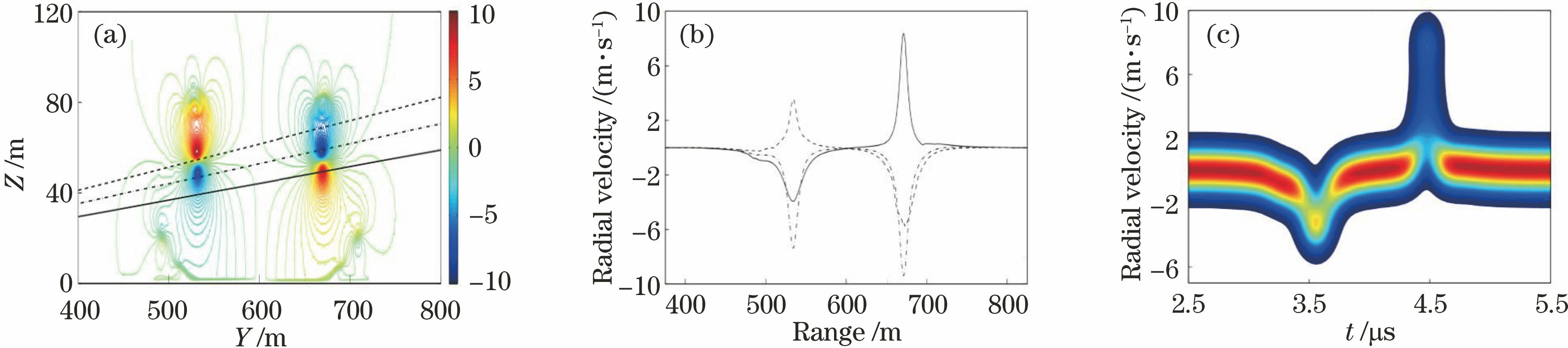
Fig. 1. Simulation results of tail vortex and Wigner-Ville distribution of radial velocity profiles. (a) Numerical simulation diagram of contour plot of tail vortex pair; (b) three radial velocity profiles of line of slight; (c) average Wigner-Ville distribution of black solid lines in fig. (b)

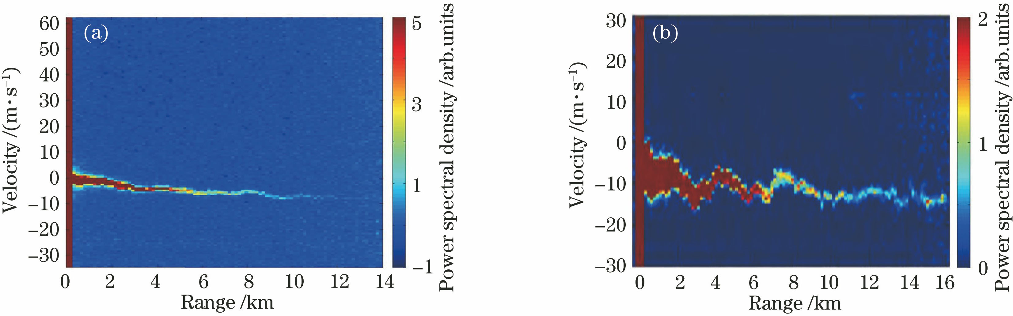
Fig. 2. Spectral images of wind speed varying with distance. (a) 1.5 μm all-fiber single frequency lidar; (b) long-distance Doppler lidar

Fig. 3. Reconstruction results of 2D wavelet. (a) Original relative temperature perturbations from July 16 to 18, 2014; (b) reconstruction period of 3.6 h; (c) reconstruction period of 4.8 h; (d) reconstruction period of 7.8 h; (e) the temperature perturbation field reconstructed from combining the above three major wave packets

Fig. 4. Gravity wave perturbations (a)-(c) and distribution function of spectral energy (d)-(f). (a) Initial temperature perturbations; (b) waves with upward phase progression; (c) waves with downward phase progression; (d) Vertical wavelength versus phase velocity; (e) vertical wavelength versus period; (f) altitude versus vertical wavelength

Fig. 5. Comparison of wind shear distribution between simulation results and actual measurements. (a) Simulation results; (b) actual measurements

Fig. 6. Comparison diagrams of inversion results. (a) Original and denoised data; (b) denoised data and average of 1000 sets of accumulative signals

Fig. 7. Spectral distribution of backscatter signals

Fig. 8. Comparison of the spectrogram results. (a) Spectrogram and oscillogram of an original LDV signal; (b) spectrogram and oscillogram of a Wiener filtered signal; (c) spectrogram and oscillogram of a clean signal

Fig. 9. THI displays of water-vapor mixing ratio recorded from 2016-09-22T00:00 to 2016-09-23T00:00 before and after denosing. (a) Before denoising; (b) after denoising

Fig. 10. Spectrograms of the received signals from the targets at 250 m. (a) Stationary target; (b) moving target

Fig. 11. Test results of Gabor wavelet transform. (a) Tile 1 original data; (b) Tile 1 segmented result; (c) Tile 2 original data; (d) Tile 2 segmented result

Fig. 12. Comparison of segmented trees and buildings using matching pursuit method. (a) Trees; (b) buildings; (c) tree area detected by an 11×11 window; (d) building area detected by an 11×11 window; (e) tree area detected by a 7×7 window; (f) building area detected by a 7×7 window

Fig. 13. Spectrogram results. (a) Normalized spectrogram of the target speed versus time with tone spacing of 10 GHz; (b) velocity spectrogram after hard threshold processing

Fig. 14. Airplane model and imaging results based on two methods. (a) Optical photo of the airplane model made of stone; (b) image result based on the FFT(fast Fourier transformation) method; (c) azimuth multilook result based on the FFT method; (d) azimuth multilook result based on the JTFT method

Fig. 15. Spectrogram of walking person

Table 1. Approximate peak to LO noise performances for continuous wave coherent lidar

Table 2. Comparison of various time-frequency analysis methods