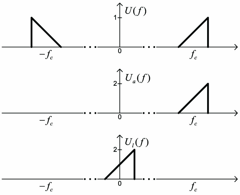
Fig. 1. Spectra of bandpass signal U(f), analytic signal Ua(f), and baseband equivalent signal Ul(f).

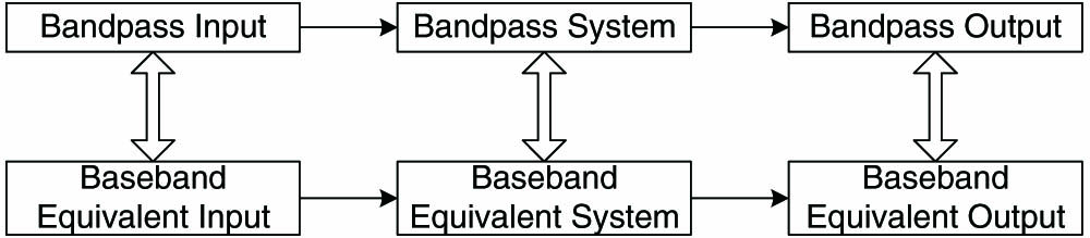
Fig. 2. Time-domain simulation of the bandpass system and baseband equivalent system.

Fig. 3. Flow chart of the proposed modeling framework for the time-domain simulation of photonic systems.

Fig. 4. Frequency ranges of Models A, LA, B, and LB.

Fig. 5. Example MZI. The geometric structure of the MZI under study.

Fig. 6. Example MZI. The electronic signal and amplitude modulated optical signal for the MZI.

Fig. 7. Example MZI. Comparison of the magnitude (top) and phase (bottom) of the MZI scattering parameters extracted via Caphe (full blue line) and Model A (red dashed line), where the green dots represent the corresponding absolute error.

Fig. 8. Example MZI. Comparison of the magnitude (left) and phase (right) of the MZI scattering parameters extracted via Caphe (full blue line) and Model LB (red dashed line), where the green dots represent the corresponding absolute error.

Fig. 9. Example MZI. The output at port P3 of the MZI, where the red line is the absolute value of the complex signal obtained by the time-domain simulation of Model LB, the blue line is the corresponding signal from Model A, and the marker × denotes the same signal from the analytic model.

Fig. 10. Example MZI. Time-domain simulation of Models LA and LB with very narrow pulse input signal. The black line is the electronic input signal, the red solid line is the output at port P3 of the analytic model, and the blue dashed line and green dotted line indicate the outputs at the same port of Models LA and LB, respectively.

Fig. 11. Example RR. The geometric structure of the double ring resonator.

Fig. 12. Example RR. Comparison of the magnitude (top) and phase (bottom) of the ring resonator scattering parameters extracted via Caphe (full blue line) and Model A (red dashed line), where the green dots represent the corresponding absolute error.

Fig. 13. Example RR. Comparison of the magnitude (left) and phase (right) of the ring resonator scattering parameters extracted via Caphe (full blue line) and Model LB (red dashed line), where the green dots represent the corresponding absolute error.

Fig. 14. Example RR. The modulating signals: in-phase part I and quadrature part Q.

Fig. 15. Example RR. The output at port P3 of the double ring resonator, where the red line is the absolute value of the complex signal obtained by the time-domain simulation of Model LB, and the blue line is the corresponding signal from Model A.

Fig. 16. Example RR. The output at port P4 of the double ring resonator. Left: the output of Model A. Right: the recovered bandpass output from Model LB.

Fig. 17. Example RR. A zoom of the output at port P4 of the double ring resonator around t=45.6  ps (the green rectangular area in Fig. 16). The blue line is used for Model A, while the red dash line is the recovered bandpass output from Model LB.

Fig. 18. Example LF. The geometric structure of the MZI lattice filter.

Fig. 19. Example LF. Pseudo-random sequence of 1000 bits for t∈[0,1] ns.

Fig. 20. Example LF. Shift of the center frequency of the passband of the lattice filter due to the tolerances of the manufacturing process.

Fig. 21. Example LF. The eye diagrams at port P4 of the baseband equivalent systems of the lattice filter with passband center frequency 195.11, 195.05, and 194.98 THz (from left to right).

Fig. 22. Spectra of bandpass system H(f), baseband equivalent system Hl(f), and baseband equivalent “shifted” system H^l(f).

Table 1. Comparison of Different Modeling Strategies

Table 2. Example MZI^a