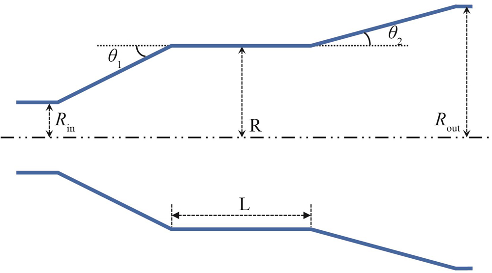
Fig. 1. The LOG cavity profile from the longitudinal view

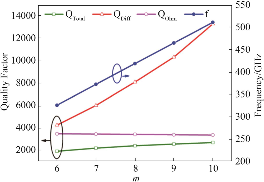
Fig. 2. The variation of the total quality factor，diffraction quality factor，ohmic loss quality factor and the oscillation frequencies of the designed modes with the azimuthal index（m）

Fig. 3. Radial distribution of the azimuthal electric field Eϕ for TEm,1 modes（m=4∼9）.ϕ and r denotes the azimuthal and radial coordinate，respectively. Jm' is the first derivative of mth order Bessel function. Rw is the waveguide radius

Fig. 4. The starting current variation with external magnetic field，where the beam voltage is 250 kV，the pitch factor is 2.0

Fig. 5. The nonlinear output power and output frequency variation with the external magnetic field

Fig. 6. Dispersion diagram of the cylindrical waveguide modes and the synchronism condition when the external magnetic field is 2.71 T and 2.76 T

Fig. 7. The nonlinear output power and output frequency variations with the beam current when the magnetic fields forTE7.1，TE8.1，TE9.1 are 2.77 T，2.74 T and 2.71 T，respectively

Fig. 8. The electric field distribution of the TE9,1,1 mode obtained by CST simulation (a) the axial electric field distribution, (b) the transverse electric field distribution

Fig. 9. The spectrum of the output signal. The inset shows the variations of the mode amplitude ofTE9,1,1 with time

Fig. 10. The output power and output frequency variations with the external magnetic field when the beam voltage is 250 kV and beam current is 3.0 A

Fig. 11. The transverse view of the electron beams when operating at different harmonics（a）the unperturbed large-orbit electron beams，（b）the azimuthal bunching at the 9^th harmonic（when B=2.71 T），（c）the azimuthal bunching at the 8^th harmonic（when B=2.73 T），（d）the azimuthal bunching at the 7^th harmonic（when B=2.77T）

Fig. 12. The output amplitude variation with time when B=2.77 T and I=3 A. The inset is the spectrum of the output signal.

Fig. 13. The output power and frequency variation with wall conductivity when B=2.72 T and I=3A.

Fig. 14. The output power and output frequency variation with the beam current when the external magnetic field is 2.71 T，2.72 T，and 2.77 T，respectively

Fig. 15. The output power variation with time when B=2.72 T and I=4.5A. The inset is the spectrum of the output signal

Table 1. The geometric parameters of the LOG cavity

Table 2. The comparison between the cold cavity analysis and hot cavity simulations