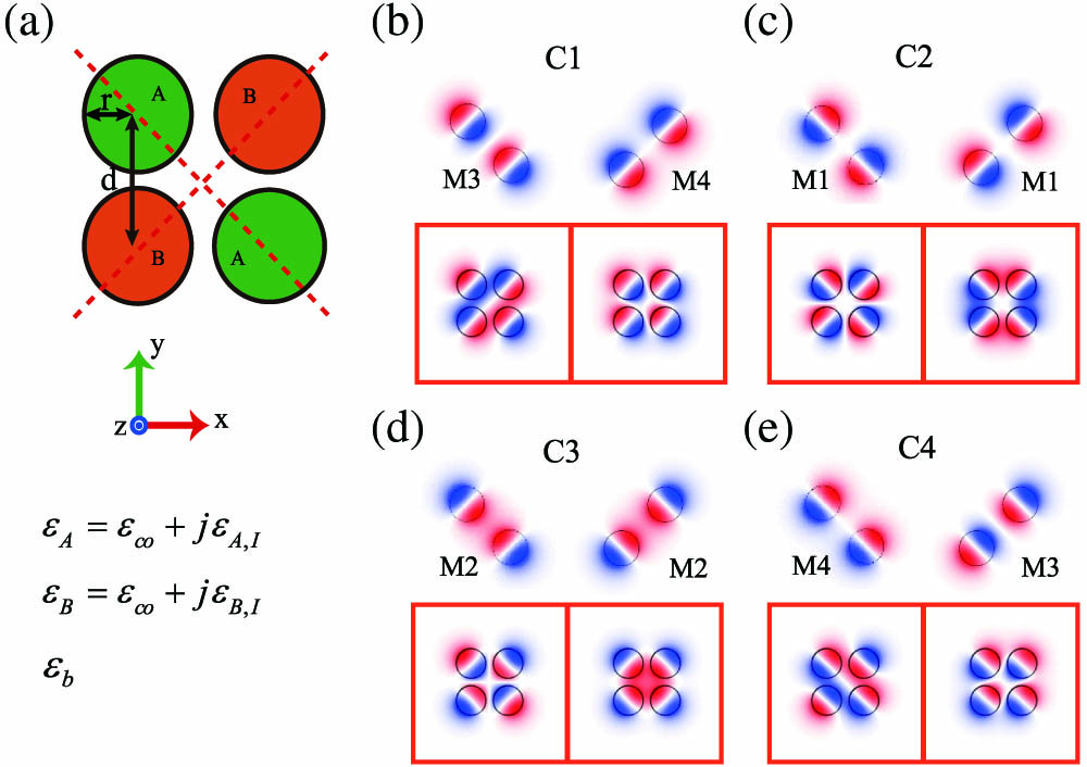
Fig. 1. Schematic of the proposed structure consisting of four coupled waveguides in a square array and the coupled-mode schemes supported in this structure. (a) Top view of the cross section profile, (b)–(e) four coupled-mode fashions between the modes supported in the diagonal (A) and off-diagonal waveguides (B). The geometrical parameters are r=0.2  μm, d=0.5  μm. The relative permittivity of the diagonal (A) waveguides and off-diagonal (B) waveguides are ϵA=ϵco+jϵA,I and ϵB=ϵco+jϵB,I, respectively. Here, ϵco=12.25 corresponds to silicon, and the background medium (silica) has the dielectric function ϵb=2.25.

Fig. 2. Propagation constants β± as a function of ϵI for different mode-coupling cases C1 (black solid curve), C2 (green solid curve), C3 (blue dashed curve), and C4 (red dashed curve). (a), (c) The real parts; (b), (d) the imaginary parts. The corresponding structure has ϵB,I=0 and ϵA,I=ϵI<0.

Fig. 3. Propagation constants as a function of ϵI for different modes supported in the diagonal (off-diagonal) waveguides: M1 (black circles, real; black solid curve, imaginary), M2 (red squares, real; red dashed curve, imaginary), M3 (green plusses, real; green solid curve, imaginary), and M4 (blue X’s, real; blue dotted curve, imaginary). (a) FEM results, (b) general CMT results. The left y axis corresponds to the real parts of the propagation constants, and the right y axis is for the imaginary parts. Here, ϵA,I=ϵI.

Fig. 4. Phase diagram in the parameter space (ϵI, α): the solid and dashed lines mark the classical CMT phase boundaries (e.g., one of the supermodes has a real-valued propagation constant) based on Eq. (2), and the symbols represent the FEM results.

Fig. 5. (a) Evolution of the intensity |aA|2 (red dashed line) and |aB|2 (black solid line) as functions of z for the initial condition that only the lossy waveguide mode aA is excited, (b) the total intensities (|aA|2+|aB|2) for the cases where the loss (red dashed line) and gain (black solid line) waveguides modes are excited. (a) and (b) show the system at the α-point (ϵI,α)=(0.6,0.0.9459); (c) and (d) are similar to (a) and (b), but for the point (ϵI,α)=(0.5,0.9459) in phase I.

Fig. 6. Propagation constant β as a function of ϵI: (a), (c), (e) the real parts; (b), (d), (f) the imaginary parts. The black solid lines correspond to the FEM results, the dashed red lines show the classical CMT results, and the symbols represent the general CMT results. The insets in (b) and (d) are zoomed-in views of the respective panels for relatively small ϵI values. (a), (b) α=0.9; (c), (d) α=1.08; (e), (f) α=1.3.

Table 1. Coupled-Mode Components and the Coefficients of the Hamiltonian in Eq. (3) for Four Combinations of Modes Coupling, i.e., Cases Shown in Figs. 1(b)–1(e)