Abstract
The exceptional point (EP) is one of the typical properties of parity–time-symmetric systems, arising from modes coupling with identical resonant frequencies or propagation constants in optics. Here we show that in addition to two different modes coupling, a nonuniform distribution of gain and loss leads to an offset from the original propagation constants, including both real and imaginary parts, resulting in the absence of EP. These behaviors are examined by the general coupled-mode theory from the first principle of the Maxwell equations, which yields results that are more accurate than those from the classical coupled-mode theory. Numerical verification via the finite element method is provided. In the end, we present an approach to achieve lossless propagation in a geometrically symmetric waveguide array.1. INTRODUCTION
Hermitian Hamiltonians with real eigenvalues and orthogonal eigenstates are generally used to describe closed (isolated) systems, while for an open system, there is the additional interaction of the states with the environment, resulting in a non-Hermitian Hamiltonian with complex eigenvalues and nonorthogonal eigenstates [1–3]. The extension of a Hermitian to a non-Hermitian Hamiltonian is generally achieved by introducing complex potentials or gain and loss [4–7]. Note that if the complex potentials have parity–time (PT) symmetry [4,8], the system experiences a phase transition from the unbroken phase to the broken one across an exceptional point (EP), where the eigenvalues and eigenstates coalesce. All these features lead to many interesting applications in various optical systems, including PT-symmetric lasers [9,10], coherent absorption [11], Bragg reflectors [12,13], nonreciprocal light transmission [14,15], and others [16–18]. Also, for passive PT-symmetric systems, through gauge transformation, the structure can behave in a PT-symmetric-like fashion [19,20]. When the nonlinearity included in these PT systems has been taken into account, it gives rise to a wide array of new phenomena. In particular, the gain saturation is unavoidable in amplifying optical waveguides [21,22].
Among various photonic structures, coupled optical waveguides provide one of the most appealing and experimentally accessible platforms for implementing the idea of PT symmetry [23,24], while for asymmetric coupling systems arising from asymmetric geometry or arbitrary gain and loss, the associated properties of PT symmetry are lost [24,25]. Yet with some subtle approaches, PT-symmetric-like properties can be recovered to a certain extent [26]. In Ref. [27], we revealed the absence of EP, even for a situation where the system apparently fulfills the PT symmetry condition with uniform gain and loss. This is ascribed to the different modes coupling together with unequal propagation constants. In addition to the different modes coupling, the detuning of the coupled modes arising from nonuniform gain and loss can also eliminate the EP, but more apparently yields lossless modes, which are of great importance for photonic signal processing.
In this paper, we present such a study and examine the evolution of propagation constants for four coupled waveguides in a square array with nonuniform gain and loss. The non-Hermitian Hamiltonian obtained from the classical coupled-mode theory (CMT) [28–30] can be used to describe the propagation dynamics; however, it fails to capture the influence of the gain and loss, particularly for heavy gain/loss involvement and for identical modes coupling. In order to deal with this problem, another well-established approach, referred to as general CMT, from the first-principle point of view, has been developed [31]. Based on this approach, a detailed description of the effect of the gain and/or loss factor on the propagation constants is illustrated. In particular, we present the conditions for the emergence of a purely real propagation constant via properly designed gain and loss distribution, utilizing the classical CMT and general CMT simultaneously. All of these are fundamentally related to the energy balance of the coupled modes in their spatial propagation channels (locations in the cross sections of the waveguide array).
Sign up for Photonics Research TOC. Get the latest issue of Photonics Research delivered right to you!Sign up now
2. TWO MODES COUPLING MODEL
We begin with a simple two-states model to describe the system that has two coupled propagation modes. The Hamiltonian is written as where is the propagation constant, and are the coupling strengths of the two modes, defines the intrinsic gain () or loss (), and represents the additional and tunable propagation constant introduced in the second mode. In Eq. (1), is the imaginary unit.
The eigenvalues of the Hamiltonian, i.e., Eq. (1), take the form Note that the gain/loss of the propagation modes are characterized by the imaginary parts of the propagation constants (obtained either from theoretical eigenvalues of Eq. (1) or from numerical full-wave simulation, such as COMSOL Multiphysics [32]). In experiments, the gain/loss may be achieved via erbium doping optically pumped with a laser beam [27]. In the nonlinear regime, the presence of gain saturation results in a mismatch with the loss. So a rational value of the gain/loss coefficient should be carefully adopted in the experiment in the linear regime, and also in the nonlinear regime, which is not discussed in this paper.
If and , the system reduces to the general PT-symmetric case, and experiences a transition from a fully real spectrum to a complex conjugate spectrum [4,8]. If , , and , the system corresponds to the passive PT symmetry case [33]. If , the system no longer has real eigenvalues, and the EP will not emerge. In this work, we mainly focus on the deviation of the propagation constants, stemming from the additional nonuniform gain and loss for the coupling of the originally identical modes, in addition to the coupling of different modes supported in the four coupled waveguides in a square array [see Fig. 1(a)].
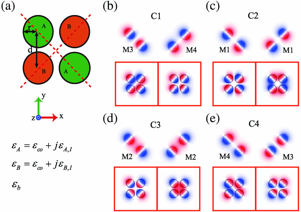
Figure 1.Schematic of the proposed structure consisting of four coupled waveguides in a square array and the coupled-mode schemes supported in this structure. (a) Top view of the cross section profile, (b)–(e) four coupled-mode fashions between the modes supported in the diagonal (A) and off-diagonal waveguides (B). The geometrical parameters are , . The relative permittivity of the diagonal (A) waveguides and off-diagonal (B) waveguides are and , respectively. Here, corresponds to silicon, and the background medium (silica) has the dielectric function .
3. FOUR COUPLED WAVEGUIDES IN A SQUARE ARRAY
To investigate and compare the two different cases (e.g., the identical mode coupling and different mode coupling cases), we consider a usual and unique structure: four coupled waveguides in a square array [27]. The Hamiltonian of this system is not transparent, as each waveguide supports two degenerate fundamental modes. To circumvent that, the system is considered as a coupled structure with supermodes supported in diagonal waveguides and the supermodes supported in off-diagonal waveguides. The supermode here refers to a hybridized mode from the fundamental ones in each individual circular waveguide. It turns out that the total structure can be represented by four isolated Hamiltonians (the modes are located in diagonal and off-diagonal waveguides), as shown in Figs. 1(b)–1(e) (respectively corresponding to coupling combinations 1–4, labeled as C1–C4). Coupling schemes C1–C4 are specific combinations of two decoupled modes (from the four modes, labeled as M1, M2, M3, and M4), supported in the diagonal and off-diagonal waveguides as shown in Figs. 1(b)–1(e), respectively.
Here, a more rigorous and systematic approach, (i.e., the nonorthogonal vector CMT based on the linear superposition of the modes for individual waveguides [30]) can be utilized to theoretically analyze the mode interactions in a two-state model. The coupled-mode equation reads where is the propagation constant for each supermode supported in diagonal (off-diagonal) waveguides, is the coupling strength, and is the corresponding normalized amplitude. denotes the gain () or loss () coefficient. Here, the wavelength is set to 1550 nm. We note that and can be calculated based on the field distribution of the decoupled modes and their overlapping integral [28,29]. The cross-interacting term is essentially treated as a complex inner product between the fields: Here, represents the normalized electric field distribution of the individual waveguide system, and is the integral cross section where waveguides are located. In this work they were obtained numerically by the finite element method (FEM) [32]. The associated coefficients, especially and , for different coupling schemes (C1–C4) are shown in Table 1, calculated by Eqs. (4) and (5). Note that are assumed to be proportional to in the conventional CMT.
| Combination | C1 | C2 | C3 | C4 |
| Diagonal | M3 | M1 | M2 | M4 |
| Off-diagonal | M4 | M1 | M2 | M3 |
| βA/k0 | 2.4842 | 2.4672 | 2.4702 | 2.4867 |
| βB/k0 | 2.4867 | 2.4672 | 2.4702 | 2.4842 |
| γA/(k0ϵA,I) | 0.1576 | 0.1641 | 0.1638 | 0.1576 |
| γB/(k0ϵB,I) | 0.1576 | 0.1641 | 0.1638 | 0.1576 |
| κA/k0 | 0.1022−0.0054j | 0.023 | 0.0187+0.0016j | 0.103 |
| κB/k0 | 0.1022+0.0054j | 0.023 | 0.0187−0.0016j | 0.103 |
Table 1. Coupled-Mode Components and the Coefficients of the Hamiltonian in Eq. (3) for Four Combinations of Modes Coupling, i.e., Cases Shown in Figs. 1(b)–1(e)
According to the eigenvalues of Eq. (3) and the coefficients in Table 1, if the permittivity of the system obeys (* stands for complex conjugate), it possesses general PT symmetry for the combinations C2 and C3, while for the other two combination schemes, the system loses the EP [27]. The absence of the EP is ascribed to the different propagation constants between the two decoupled supermodes, which originate in the intrinsic properties of the structure.
Up to now, we have considered the cases of uniform gain and loss distributions briefly. But for nonuniform gain and loss, particularly for and , which are analogous to passive PT symmetry [33], two of the total coupling cases (C2 and C3) should experience a similar transition from an unbroken phase with identical eigenvalues to a broken phase with unequal ones, according to Eq. (3), based on the classical CMT.
The corresponding numerical results obtained from FEM simulation are shown in Fig. 2 for varying amounts of gain and loss. Although they are not consistent with the above prediction, we will carefully demonstrate the reason. Note that the EPs of all four of these combinations are lost. However, after a critical amount of loss is added, the total transmission of the waveguide array increases, even though the loss amount is increased. This is similar to the passive PT symmetry, leading to loss-induced transmission [34].

Figure 2.Propagation constants as a function of for different mode-coupling cases C1 (black solid curve), C2 (green solid curve), C3 (blue dashed curve), and C4 (red dashed curve). (a), (c) The real parts; (b), (d) the imaginary parts. The corresponding structure has and .
4. ANALYSIS BASED ON GENERAL COUPLED-MODE THEORY
The CMT presented in Section 3 is valid for a definite and conserved optical power of the whole system [30], while for non-Hermitian systems with arbitrary gain and loss, and especially for systems with strong gain/loss, the total integrated power is not a conserved quantity [31]. Thus, a general CMT analysis is necessary to deal with these non-Hermitian systems. This method is based on the variational principles, in which the scalar inner product for non-Hermitian systems is used [31].
In this section, we briefly outline the theoretical procedure for constructing the general CMT; for further details, see [31,35]. We assume that the forward () propagation modes supported in the unperturbed systems are expressed as . The corresponding adjoint fields, i.e., the backward () propagation modes are . The relationships between the fields are as follows: , , , and . Here () is the vector electric (magnetic) field in the transverse cross section for forward (+) and backward (−) propagation. Importantly, the counterpropagating modes ( and ) have a definite relationship, so one can be deduced from the other. The subscript denotes the index of the supported supermodes.
The normalized forward fields satisfy the Maxwell equations where and , , and are unit vectors. When a small perturbation () is taken into account, the fields of the perturbed system can be approximately written as a linear combination of the unperturbed adjoint fields, i.e., Here, they also satisfy the Maxwell equations By considering only the effect of the perturbation, we can take certain operations of Eq. (6) multiplied by minus Eq. (10) multiplied by , and Eq. (7) multiplied by minus Eq. (11) multiplied by (instead of multiplying by the complex conjugate of the fields); then, taking the integral operator over the transverse cross section, the equation finally can be simplified to The coefficients in Eq. (12) are as follows: For the unperturbed situation (), it is easy to have . As a result, Eq. (12) reduces to Equation (16) can be rewritten as an eigenvalue problem, where , , and . The eigenvalue of the Hamiltonian is the propagation constant of the propagating modes, and the corresponding eigenvector denotes the proportion of the decoupled modes (i.e., the unperturbed modes) written as Eqs. (8) and (9). As a consequence, the propagation constant is the result of the original unperturbed modes coupling due to the involved perturbation. This is the key equation referred to as the general CMT.
In view of Eq. (16), a small perturbation has a great effect on the final propagation constants. We would utilize the general CMT to analyze the evolution of the propagation constants for the cases shown in Figs. 2(c) and 2(d). Intuitively, it comes from the detuned due to the nonuniform gain and loss for the coupling modes. In the preceding section, it was mentioned that the Hamiltonian was considered as the coupled modes formed in the diagonal and off-diagonal waveguides, and therefore we would particularly examine the evolution of each mode supported in the diagonal waveguides when the imaginary part of the permittivity is introduced. Here, the four modes (labeled as M1, M2, M3, and M4) are exactly orthogonal for the corresponding Hermitian system. As such, they are treated as single-mode interactions in the general CMT, i.e., in Eq. (16). In this case, Eq. (16) becomes Here corresponds to modes M1, M2, M3, and M4, respectively. The propagation constant after perturbation can be calculated step by step through the fields obtained by numerical simulation based on the FEM. The results are shown in Fig. 3. It is obvious that as the imaginary part of the permittivity () increases from zero, the real part of the propagation constants increases, and the increasing speed accelerates, while the imaginary part keeps growing linearly. We note that the real part is even and the imaginary part is odd with respect to . The results of the FEM agree well with the general CMT. Figure 3 further shows that the imaginary part of the permittivity has great influence on the real part of the propagation constants, especially for large values. This is the main cause of the introduction of for the coupled modes, which is responsible for the results in Figs. 2(c) and 2(d). The emergence of zero is also the reason for the formation of PT symmetry with uniform gain and loss.
Figure 3.Propagation constants as a function of for different modes supported in the diagonal (off-diagonal) waveguides: M1 (black circles, real; black solid curve, imaginary), M2 (red squares, real; red dashed curve, imaginary), M3 (green plusses, real; green solid curve, imaginary), and M4 (blue X’s, real; blue dotted curve, imaginary). (a) FEM results, (b) general CMT results. The left axis corresponds to the real parts of the propagation constants, and the right axis is for the imaginary parts. Here, .
5. REALIZATION OF STABLE PROPAGATION
According to the above analysis and the results presented in Fig. 3, it is possible to achieve a stable propagation mode (without any attenuation and amplification during the propagation) in systems with nonuniform gain and loss distributions. Lossless propagation modes are ubiquitous in PT-symmetric systems, for example, in coupled waveguides with balanced gain and loss below the EP, and attenuation is frequently encountered in the absence of PT symmetry. In this section, we show the possibility of achieving purely real eigenvalues in waveguide systems with nonuniform gain and loss, combining the classical CMT and the general CMT. Here, we use the coupling combination C1 as the example, and the results can be applied to the other cases (e.g., C2, C3, and C4).
To simplify the discussion, we introduce the degree of freedom (, ). A stable propagation mode requires that . By inserting into Eq. (3) the parameters (listed in Table 1) obtained from the classical CMT, we get a phase diagram describing the properties of the mode coupling (M3 and M4) as shown in Fig. 4, where the black solid line corresponds to the case of , representing one lossless eigenstate and one lossy one. Notice that the red dashed line corresponds to , for which the system has a gain eigenstate and a lossless one. For parameters in the black and the red lines, the system is tuned to a point (let us call it the ‘- point’ for convenience) where one of the two supermodes we considered conserves its energy during propagation. For this reason, the whole parameter space is separated into three regions labeled I, II, and III in Fig. 4. It is easy to see that region I consists of double lossy eigenstates, region II has a gain eigenstate and a lossy one, and region III contains two gain eigenstates. Importantly, we can see that there exist two independent solutions for (for a certain value range) and a single solution for . Also, there exists a limit for the choice of to fulfill . Thus, the properties of the entire system can be distinguished by the specific parameter pair (, ). The propagation behaviors of the system are then discussed in some detail, essentially using Fig. 4 as a rough guideline. The numerical results for a purely real propagation constant are also shown in Fig. 4 with different symbols (circles and squares).
Figure 4.Phase diagram in the parameter space (, ): the solid and dashed lines mark the classical CMT phase boundaries (e.g., one of the supermodes has a real-valued propagation constant) based on Eq. (2), and the symbols represent the FEM results.
To check the detailed modal properties, we first focus on a specific -point of , which falls right on the black solid curve in Fig. 4. With these settings, the system supports two supermodes: one of effective index and the other of . To see the consequence of such a nonuniform combination of gain and loss, we use the fourth-order Runge–Kutta method to solve Eq. (3). Figure 5 shows the evolution of the slowly varying intensity () as a function of the propagation distance . This is for the case when the lossy waveguide mode is initially excited. It is seen that the optical field is able to be coupled into the gain waveguide mode . There is also obvious beam oscillation for both modes, resulting from the interference of the asymmetric mode and their reciprocal coupling. The oscillation period is determined by the mismatch of the real parts of the supermode refractive indices as , where . Alternatively, for the case of the initial excitation of the gain waveguide mode , there is similar propagation behavior.
Figure 5.(a) Evolution of the intensity (red dashed line) and (black solid line) as functions of for the initial condition that only the lossy waveguide mode is excited, (b) the total intensities () for the cases where the loss (red dashed line) and gain (black solid line) waveguides modes are excited. (a) and (b) show the system at the -point ; (c) and (d) are similar to (a) and (b), but for the point in phase I.
For another particular pair , which falls into the phase region I in Fig. 4, similar beam oscillation can be observed [see Figs. 5(c) and 5(d)]. However, the optical field propagation suffers from overall attenuation, decaying approximately to zero after a distance . For this system, the two supermodes are both lossy, in agreement with the phase diagram in Fig. 4. It is noted that the attenuation at relatively small values in region I is quite small, which indicates that light can propagate over long distances (in the order of millimeters).
We emphasis that the differences between the results of classical CMT and FEM in Fig. 4 are partially due to the fact that the coefficients in Table 1 are obtained by the original field distributions of the corresponding Hermitian system. This treatment neglects the perturbation of mode profile and coupling by including the imaginary part of the permittivity. To have a clearer and more exact theoretical modeling, the abovementioned general CMT in Section 4 is applied here. Our system can be represented by a two-mode coupling model, so based on Eq. (16), the corresponding general coupled-mode equation can be written as Here, the perturbation is (diagonal waveguides) and (off-diagonal waveguides).
Figure 6 shows the corresponding results from the FEM, the classical CMT, and the general CMT. For different values, the results of the FEM and general CMT all agree quite well. When increases from the loss-dominated value () to the gain-dominated value (), the real parts of the two bands approach, and the imaginary parts experience a transition, meaning that the system goes from two lossy eigenstates to two gain ones. This exactly illustrates and corroborates the phase region partition in Fig. 4. For at , there exist two choices of , and the corresponding dispersion relations are shown in Figs. 6(c)–6(f). This clearly demonstrates the difference between the selection of and in order to have a stable mode. Despite the very good agreement with respect to the FEM results, we note that the general CMT could not directly provide a phase boundary prediction as shown in Fig. 4, while the classical CMT can give a rough estimation of these phase boundaries. Therefore, the classical CMT and the general CMT can be complementary to each other in terms of verification and prediction, apart from brute force numerical methods.
Figure 6.Propagation constant as a function of : (a), (c), (e) the real parts; (b), (d), (f) the imaginary parts. The black solid lines correspond to the FEM results, the dashed red lines show the classical CMT results, and the symbols represent the general CMT results. The insets in (b) and (d) are zoomed-in views of the respective panels for relatively small values. (a), (b) ; (c), (d) ; (e), (f) .
In conclusion, we have revealed the eigenvalue dynamics for a system of four geometry identical waveguides with nonuniform gain and loss. Based on the first principle of the Maxwell equations, the general CMT is used to understand the origin of the offset of originally equal propagation constants in the presence of permittivity perturbation, especially for the real part. The offset leads to asymmetric mode coupling and the absence of EP. Also, the system can be tuned to support supermodes with real propagation constants, via a carefully designed gain/loss ratio in the individual waveguides. We show that such a system has a phase transition that interfaces two regimes: one with both coupled propagation modes being lossy, the other with one gain and one lossy mode. It can also be optimized to demonstrate a different transition from the phase with all gain states to a phase with one gain and one lossy. The required tuning parameter is the gain/loss ratio : for the former, , while for the latter, . The additional degree of freedom is introduced to modify the energy distribution, in order to compensate the mode asymmetry-induced imbalance. It is noted that closely relies on the propagation constant of the decoupled modes. Furthermore, our results may be extended to plasmonic or plasmonic–dielectric hybridized waveguide systems.
References
[1] C. M. Bender. Making sense of non-Hermitian Hamiltonians. Rep. Prog. Phys., 70, 947-1018(2007).
[2] N. Moiseyev. Non-Hermitian Quantum Mechanics(2011).
[3] I. Rotter. A non-Hermitian Hamilton operator and the physics of open quantum systems. J. Phys. A, 42, 153001(2009).
[4] C. M. Bender, S. Boettcher. Real spectra in non-Hermitian Hamiltonians having PT symmetry. Phys. Rev. Lett., 80, 5243-5246(1998).
[5] K. G. Makris, R. El-Ganainy, D. N. Christodoulides, Z. H. Musslimani. Beam dynamics in PT symmetric optical lattices. Phys. Rev. Lett., 100, 103904(2008).
[6] R. El-Ganainy, K. G. Makris, D. N. Christodoulides, Z. H. Musslimani. Theory of coupled optical PT-symmetric structures. Opt. Lett., 32, 2632-2634(2007).
[7] B. Peng, Ş. K. Özdemir, S. Rotter, H. Yilmaz, M. Liertzer, F. Monifi, C. M. Bender, F. Nori. Loss-induced suppression and revival of lasing. Science, 346, 328-332(2014).
[8] C. E. Rüter, K. G. Makris, R. El-Ganainy, D. N. Christodoulides, M. Segev, D. Kip. Observation of parity-time symmetry in optics. Nat. Phys., 6, 192-195(2010).
[9] L. Feng, Z. J. Wong, R.-M. Ma, Y. Wang, X. Zhang. Single-mode laser by parity-time symmetry breaking. Science, 346, 972-975(2014).
[10] H. Hodaei, M. Miri, M. Heinrich, D. N. Christodoulides, M. Khajavikhan. Parity-time symmetric microring lasers. Science, 346, 975-978(2014).
[11] Y. Sun, W. Tan, H. Li, J. Li, H. Chen. Experimental demonstration of a coherent perfect absorber with PT phase transition. Phys. Rev. Lett., 112, 143903(2014).
[12] M. Kulishov, B. Kress. Free space diffraction on active grating with balanced phase and gain/loss modulation. Opt. Express, 20, 29319-29328(2012).
[13] Z. Lin, H. Ramezani, T. Eichelkraut, T. Kottos, H. Cao, D. N. Christodoulides. Unidirectional invisibility induced by PT-symmetric periodic structure. Phys. Rev. Lett., 106, 213901(2011).
[14] B. Peng, S. K. Ozdemir, F. Lei, F. Monifi, M. Gianfreda, G. L. Long, S. Fan, F. Nori, C. M. Bender, L. Yang. Nonreciprocal light transmission in parity-time-symmetric whispering-gallery microcavities. Nat. Phys., 10, 394-398(2014).
[15] L. Chang, X. Jiang, S. Hua, C. Yang, J. Wen, L. Jiang, G. Li, G. Wang, M. Xiao. Parity-time symmetry and variable optical isolation in active-passive-coupled microresonators. Nat. Photonics, 8, 524-529(2014).
[16] S. V. Suchkov, S. V. Dmitriev, B. A. Malomed, Y. S. Kivshar. Wave scattering on a domain wall in a chain of PT-symmetric couplers. Phys. Rev. A, 85, 033825(2012).
[17] H. Benisty, A. Lupu, A. Degiron. Transverse periodic PT symmetry for modal demultiplexing in optical waveguides. Phys. Rev. A, 91, 053825(2015).
[18] A. Regensburger, C. Bersch, M. A. Miri, G. Onishchukov, D. N. Christodoulides, U. Peschel. Parity-time synthetic photonic lattices. Nature, 488, 167-171(2012).
[19] A. Guo, G. J. Salamo, D. Duchesne, R. Morandotti, M. Volatier-Ravat, V. Aimez, G. A. Siviloglou, D. N. Christodoulides. Observation of PT symmetry breaking in complex optical potentials. Phys. Rev. Lett., 103, 093902(2009).
[20] M. Kang, F. Liu, J. Li. Effective spontaneous PT-symmetry breaking in hybridized metamaterials. Phys. Rev. A, 87, 053824(2013).
[21] A. U. Hassan, H. Hodaei, M. A. Miri, M. Khajavikhan, D. N. Christodoulides. Nonlinear reversal of the PT-symmetric phase transition in a system of coupled semiconductor microring resonators. Phys. Rev. A, 92, 063807(2015).
[22] X. Zhou, Y. D. Chong. PT symmetry breaking and nonlinear optical isolation in coupled microcavities. Opt. Express, 24, 6916-6930(2016).
[23] N. X. A. Rivolta, B. Maes. Symmetry recovery for coupled photonic modes with transversal PT symmetry. Opt. Lett., 40, 3922-3925(2015).
[24] C. Ma, W. Walasik, N. M. Litchinitser. Meta-PT symmetry in asymmetric directional couplers(2015).
[25] S. Nixon, J. Yang. All-real spectra in optical systems with arbitrary gain-and-loss distributions. Phys. Rev. A, 93, 031802(2016).
[26] S. N. Ghosh, Y. D. Chong. Exceptional points and asymmetric mode switching in plasmonic waveguides. Sci. Rep., 6, 19837(2015).
[27] Z. Liu, Q. Zhang, X. Liu, Y. Yao, J. J. Xiao. Absence of exceptional points in square waveguide arrays with apparently balanced gain and loss. Sci. Rep., 6, 22711(2016).
[28] S. Zheng, G. Ren, Z. Lin, S. Jian. Mode-coupling analysis and trench design for large-mode-area low-cross-talk multicore fiber. Appl. Opt., 52, 4541-4548(2013).
[29] K. Okamoto. Fundamentals of Optical Waveguides(2006).
[30] W. P. Huang. Coupled-mode theory for optical waveguides: an overview. J. Opt. Soc. Am. A, 11, 963-983(1994).
[31] J. Xu, Y. T. Chen. General coupled mode theory in non-Hermitian waveguides. Opt. Express, 23, 22619-22627(2015).
[32] .
[33] K. Ding, G. Ma, M. Xiao, Z. Q. Zhang, C. T. Chan. Emergence, coalescence, and topological properties of multiple exceptional points and their experimental realization. Phys. Rev. X, 6, 021007(2016).
[34] A. Cerjan, S. Fan. Eigenvalue dynamics in the presence of non-uniform gain and loss. Phys. Rev. A, 94, 033857(2016).
[35] B. Wu, B. Wu, J. Xu, J.-J. Xiao, Y. Chen. Coupled mode theory in non-Hermitian optical cavities. Opt. Express, 24, 16566-16573(2016).


