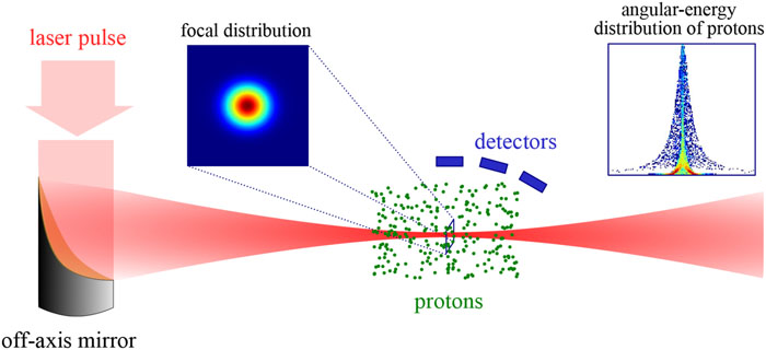
Fig. 1. Main scheme of laser pulse diagnostics via the angular spectral distributions of protons accelerated from the focus of the measured laser pulse.

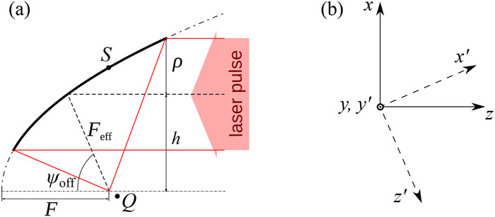
Fig. 2. (a) Scheme for focusing a laser pulse by an off-axis parabolic mirror. F and F_eff are the parent and effective focal lengths, ψ_off is the off-axis angle, and ρ is the mirror radius. (b) Coordinate systems used in this work, taking into account the positions in the scheme (a).

Fig. 3. (a1) and (a2) Focal intensity profiles for a tightly focused Gaussian beam with f_# = 0.70, D_F = 1.0λ, and z_R = 4.3λ and for a tightly focused Laguerre–Gaussian beam with f_# = 1.05, D_F = 1.0λ, and z_R = 17.8λ, respectively. (b1) and (b2) Longitudinal intensity profiles for these Gaussian and Laguerre–Gaussian beams, respectively; temporal profiles are not taken into account in these plots. Note the substantial degree of asymmetry resulting from tight focusing by an off-axis parabolic mirror. (c1) and (c2) ϕ-integrated spectral distributions of protons for the Gaussian and Laguerre–Gaussian beams, respectively. The vertical and horizontal axes as well as the color axis are the same for each image pair (a1) and (a2), (b1) and (b2), and (c1) and (c2).

Fig. 4. (a1) and (a2) Spatial distributions of the squared gradient of the normalized spatial intensity profile g(r⃗) in the xz plane for the tightly focused Gaussian and Laguerre–Gaussian beams, respectively. (b1) and (b2) ϕ-integrated spectral distributions of protons, with a logarithmic scale on the energy axis for the Gaussian and Laguerre–Gaussian beams, respectively. The red rectangles outline the low-energy parts, where the presence of the secondary ring manifests itself for the Laguerre–Gaussian beam. The vertical and horizontal axes as well as the color axes are the same for each image pair (a1) and (a2), and (b1) and (b2).

Fig. 5. (a) ϕ, θ-integrated spectral distributions of protons accelerated by tightly focused Gaussian (blue line) and Laguerre–Gaussian (red line) beams. The parameters of the Gaussian beam are f_# = 0.70, D_F = 1.0λ, and z_R = 4.3λ, while those for the Laguerre–Gaussian beam are f_# = 1.05, D_F = 1.0λ, and z_R = 17.8λ. (b1) Cutoff (maximum) energy as a function of squared maximum intensity gradient ([∇⃗g(r⃗)]max)2, where g(r⃗) is the normalized spatial distribution of the intensity. The maximum intensities at the focal spot for all data points are set to 10²² W cm⁻². The green, blue, and red dots show the data for flat-top, Gaussian and Laguerre–Gaussian profiles, respectively; the black line shows the linear approximation Emax∼([∇⃗g(r⃗)]max)2. (b2) The same as (b1), but with the maximum intensities set to 10²³ W cm⁻².

Fig. 6. (a) Scheme of the CNN architecture with two convolutional layers (“Conv2D”) with ReLU activation function, followed by pooling layers (“MaxPool2D”) and one fully connected (“Dense”) layer with 100 neurons and sigmoid activation function. The input data are 100 × 100 grayscale images of ϕ-integrated proton spectra, and the output data are 200 × 200 grayscale images of intensity distribution. (b) Example of learning curves obtained in one of the training runs and showing the decrease in the root-mean-square prediction error with the number of iterations for the training (blue curve) and validation (orange curve) data sets.

Fig. 7. CNN predictions made on a test data set containing solely cases not present in the training or validation data set. As the intensity distributions are axially symmetric, for ease of comparison only radial profiles are shown. Black lines show correct profiles, and blue markers the CNN predictions. Note that in some cases these are indistinguishable from one another. (a1)–(a3) Flat-top profiles with {f_# = 1.3, I₀ = 2 × 10²² W cm⁻²}, {f_# = 2.8, I₀ = 3 × 10²¹ W cm⁻²}, and {f_# = 3.3, I₀ = 6 × 10²¹ W cm⁻²}, respectively; the total number of particles is N_tot = 10⁴. (b1)–(b3) Gaussian profiles with {f_# = 1.4, I₀ = 8 × 10²¹ W cm⁻²}, {f_# = 2.2, I₀ = 1.3 × 10²² W cm⁻²}, and {f_# = 2.6, I₀ = 4 × 10²¹ W cm⁻²}, respectively; the total number of particles is N_tot = 10⁴. (c1)–(c3) Laguerre–Gaussian profiles with {f_# = 2.1, I₀ = 3 × 10²¹ W cm⁻²}, {f_# = 2.9, I₀ = 1.6 × 10²² W cm⁻²}, and {f_# = 3.5, I₀ = 3 × 10²² W cm⁻²}, respectively; the total number of particles is N_tot = 7 × 10⁴. The vertical and horizontal axes are the same for all plots. (d1) and (d2) Comparison of the correct two-dimensional intensity distribution with the two-dimensional profile retrieved by the CNN; the parameters of the laser beam correspond to (b2).

Fig. 8. (a1) and (a2) Comparison of the ϕ-integrated proton spectra obtained for N_tot = 10⁴ particles and N_tot = 3 × 10³ particles, respectively. (b1) and (b2) Corresponding radial intensity profiles predicted by the CNN. Black lines show correct profiles, and blue markers show CNN predictions. Note that despite the threefold decrease in the number of particles in (a2), the intensity profile (b2) is still retrieved correctly. The vertical and horizontal axes are the same for each of the image pairs (a1) and (a2), (b1) and (b2), as are the color axes for (a1) and (a2).

Fig. 9. (a) Focal intensity profile for an elliptic beam produced by tight focusing of a Gaussian beam with an off-axis mirror, half of which was covered by an aperture. (b) ϕ-integrated spectral distribution of protons for this elliptic beam. (c) Spectral distribution of protons accelerated along the ellipse’s major axis with ϕ = (0.0 ± 1.0)°. (d) Spectral distribution of protons accelerated along the ellipse’s minor axis with ϕ = (90.0 ± 1.0)°.

Fig. 10. (a) Radial intensity profiles along the direction ϕ = 0°: correct (black curve) and predicted on the basis of ϕ-integrated spectral distribution of protons (blue curve). (b) Radial intensity profiles along the direction ϕ = 90°: correct (black curve) and predicted on the basis of ϕ-integrated spectral distribution of protons (blue curve). (c) Same as (a), but with the prediction made on the basis of the ϕ = (0.0 ± 1.0)° segment of the spectral distribution. (d) Same as (b), but with the prediction made on the basis of the ϕ = (90.0 ± 1.0)° segment of spectral distribution.

Table 1. Summary of the CNN predictions made on the basis of ϕ-integrated proton spectra with different numbers of particles for three different intensity profiles: flat-top (FT), Gaussian (G), and Laguerre–Gaussian (LG). Note that to ensure that the particle density was approximately the same in all cases, a higher number of particles was used for the Laguerre–Gaussian profiles than for the flat-top and Gaussian profiles.