
N. D. Bukharskii, O. E. Vais, Ph. A. Korneev, V. Yu. Bychenkov. Restoration of the focal parameters for an extreme-power laser pulse with ponderomotively scattered proton spectra by using a neural network algorithm[J]. Matter and Radiation at Extremes, 2023, 8(1): 014404
- Matter and Radiation at Extremes
- Vol. 8, Issue 1, 014404 (2023)
Abstract
I. INTRODUCTION
Progress in the development of high-power laser technology has enabled the construction of laser facilities with laser beam power exceeding the petawatt (PW) level.1 After tight focusing, laser pulses generated by such systems may achieve extreme peak intensities of 1022 W cm−2 and higher. Although the number of PW class facilities is gradually increasing, achieving ultrahigh peak intensities remains a difficult technical challenge. In 2004, a peak intensity of 1022 W cm−2 was demonstrated on the 0.3 PW HERCULES facility (USA),2 and, after an upgrade, this record was surpassed by an intensity of 2 × 10²² W cm−2.3 It was a long time before similar results could be achieved elsewhere. Only toward the end of the last decade were intensities exceeding 1022 W cm−2 obtained on the 0.3 PW J-KAREN-P (Japan),4 Texas PW (USA),5 4.0 PW CoReLS (South Korea),6 and 5.4 PW SULF (China)7 facilities. More recently, in 2021, with careful wavefront control, a higher peak intensity exceeding 1023 W cm−2 was reported on CoReLS.8 With these increasing intensities, their measurement is becoming more and more important and challenging, owing to the many concurrent processes that occur in the highly nonlinear regime of extreme intensity.
A rough method of measurement is to estimate the peak laser intensity based on the peak laser power P0, which can be calculated knowing the total energy contained in the laser pulse and its temporal profile. The peak intensity I0 may then be obtained for a given spatial distribution of the laser beam in the focal plane I(r) = I0f(r) as
Several methods have been proposed in this context, including the use of multiple tunneling ionization of high-Z atoms with high ionization potentials,9–11 nonlinear Compton/Thomson scattering,12–19 electron–positron pair production,20 and ponderomotive scattering of electron bunches.21 Some of these can be used to diagnose other pulse parameters (such as pulse duration and focal spot size) along with the peak intensity estimation. To achieve the desired accuracy with the proposed methods proposed, certain difficulties need to be overcome. While the major problem of the multiple tunneling ionization method at intensities above 1022 W cm−2 is the importance of ponderomotive acceleration of high-Z ions in the laser field, the other approaches mentioned require perfect synchronization and spatial overlap of both particle and laser beams, as well as full characterization of the electron beam. At the same time, achieving the highest laser intensity requires tight focusing of the laser pulse, which results in strong gradients of the ponderomotive force that can accelerate even some heavy particles without synchronized pre-acceleration. The resulting angular energy distributions contain information about the laser pulse parameters, which in principle may be extracted as a solution of an inverse problem. There have been some investigations considering electrons as detecting particles,22–28 but, for a tightly focused laser pulse with high peak intensity, electrons are expelled from the focal volume before interaction with the main laser peak, which is one of the main disadvantages of this approach for full laser pulse characterization. In a recent work,29 it has been proposed to use protons for diagnostic purposes in the case of laser pulses with intensity from 1021 to 1024 W cm−2. A further development of this method is to use both types of particles (i.e., protons and electrons),30 which makes it possible to simultaneously estimate the peak intensity of a high-power laser pulse, the size of its focal spot, and its duration. In this work, we address the principal approaches to the inverse problems of focal parameter reconstruction for a tightly focused extremely intensive laser beam, based on ponderomotively accelerated protons.
Although, as mentioned above, some methods may be applied to estimate several laser parameters, they need information concerning the spatial–temporal distribution of the laser pulse, because of the dependence of the results on the focal laser distribution.28,31 It has been shown28 that the form of the electron energy spectrum depends on the focal distribution of the laser beam. Similarly, some relationship is expected between the distributions of accelerated protons and laser profiles that are studied in this paper. The inverse problem of reconstruction of laser focal profiles based on particle angular energy distributions, in turn, may be targeted with use of an artificial neural network (ANN). Here, we use convolutional neural network (CNN) architectures, which have gained wide recognition as useful tools for computer vision and image analysis tasks.32,33 Moreover, with the development of deep CNNs, such architectures have become the dominant approach for almost all recognition and detection tasks and are approaching human performance.34 In addition to general technical tasks (e.g., face and text recognition), they have also been widely used to solve various classification and regression problems in physical sciences.35–42
This article focuses on the interplay between the physics of proton dynamics in the extremely highly focused electromagnetic field and the key featured imprints on the obtained spectra, with the aim of reconstructing both the laser intensity distribution and the peak value in the focal region. In our previous work,29 we have already shown that in the regime of nonrelativistic proton acceleration, the angular characteristics of proton distributions depend on the focal spot size, while their energy characteristics are also determined by the pulse peak intensity and its duration. It has been pointed out that a nonisotropic distribution of the laser intensity in the focal plane leads to nonisotropic proton spectra, i.e., the dependence of the laser spatial distribution on the polar angle results in a corresponding dependence of the particle distribution. At the same time, the important question of how the dependence of the laser spatial distribution on the radius in the focal plane impacts on the proton distributions has not been considered, while non-Gaussian focal distributions with different energies in diffraction half-rings are sometimes observed in experiments.6,7 To analyze this effect, here, for the purpose of demonstration, we consider axially symmetric laser beams. As in our previous work,29 the proton dynamics are calculated using the nonrelativistic ponderomotive force approximation,43 and the laser pulses are simulated by Stratton–Chu integrals,44 which model laser beams with different spatial profiles focused by an off-axis parabolic mirror down to the diffraction limit. As shown in Ref. 29, in a certain range of laser intensities and focal spot sizes, the proton angular energy distribution can be scaled based on a simple expression. In this range, this allows us to prepare an augmented dataset using data calculated for only one intensity value for each focal spot size and spatial distribution. Using such a dataset, we present a neural network approach that enables reconstruction of the laser pulse focal distribution (including its quantitative characteristics such as focal spot size) as well as the laser peak intensity using the angular energy distributions of the particles. We use the calculated angular energy distributions and focal spatial profiles as samples for ANN training and testing. Although our approach is tested here for axially symmetric beams, it can be applied in more general cases with changes in the shape of the input data covering additional variables upon which the focal distribution may depend, such as the polar angle ϕ.
II. PROTON DYNAMICS IN THE FIELD OF TIGHTLY FOCUSED LASER PULSES WITH DIFFERENT SPATIAL PROFILES
The method presented in this paper for reconstructing the intensity profile of a laser pulse is based on analysis of the angular energy distributions of protons after their acceleration by the diagnosed tightly focused laser beam. Figure 1 shows the main setup of this laser diagnostic method. A laser pulse focused by an off-axis parabolic mirror interacts with protons from a rarefied gas, after which those particles expelled from the focal volume are detected at certain angles counted from the direction of laser propagation, and their angular energy distributions are used to predict the focal profile of the laser beam and its peak intensity. Such a diagnostic approach is possible if the distribution of particles is determined by the parameters of the laser pulse. This limits the parameters of diagnostic gases by neglecting the effects of both the interaction of protons with the volume of the residual charge (after expelling electrons) and multiple proton scattering due to collisions of protons with hydrogen nuclei (ion–ion collisions). Both factors have been discussed in detail in Ref. 29.
![]()
Figure 1.Main scheme of laser pulse diagnostics via the angular spectral distributions of protons accelerated from the focus of the measured laser pulse.
We recall the main expressions for estimating the experiment parameters to satisfy the conditions for applicability of the method. The first effect is related to the insignificance of the Coulomb interaction of an individual proton with the volume charge compared with the ponderomotive force of the laser pulse. In this case, the proton concentration is limited by
A. Models used to simulate the interaction of a particle with a laser pulse
Following the general approach presented in Ref. 29, we use the approximation of a nonrelativistic ponderomotive force to describe the interaction of a proton with a laser pulse whose intensity is in the extreme range from 1021 to 1024 W cm−2:
We let the incident laser pulse propagate along the z axis and take the origin of the coordinate system at the position of the parabola focus, and thus the electric field of the laser pulse focused by the mirror (with radius ρ, off-axis angle ψoff, and parent parabola focal length F) is represented as
![]()
Figure 2.(a) Scheme for focusing a laser pulse by an off-axis parabolic mirror.
We neglect border effects from the mirror edge, as well as the influence of the temporal profile on the laser spatial distribution. The former is possible for mirrors with a large focal length F of the parent mirror compared with the laser wavelength, i.e., kF ≫ 1,49 and although spatial–temporal couplings must be taken into account to simulate single- or few-cycle tightly focused laser pulses,50–52 these remain beyond the ranges discussed in this article.
In this paper, we demonstrate the robustness of the proposed method while applying it to laser pulses linearly polarized along the x axis (hereinafter, we omit the primes on the coordinates: x′, y′, z′) with a Gaussian temporal profile and a FWHM duration of 30 fs and one of the following spatial profiles: flat-top, Gaussian distributions of the second, fourth, and sixth orders, and the Laguerre–Gaussian mode
Using the above laser configuration, we calculate the final energies and the emission angles of protons, which were initially at rest, by independently integrating Eq. (1) by the Adams method.53 With axially symmetric laser beams, the final distribution of accelerated particles also does not depend on the polar angle in the xy plane ϕ, measured from the direction of laser polarization.29 Note that the use of axially symmetric beams in this example facilitates the analysis, although it is not demanded by the method itself, which, with certain modifications of the training data set, namely, considering more general asymmetric cases, can be used to assess more complex beams with no axial symmetry. With polar-angle symmetry, we consider θE distributions of particles, where E is the final proton energy and θ is the azimuth angle between the particle emission direction and the z axis.
B. Influence of the distribution of the laser pulse near its focus on proton dynamics
The laser intensity distribution in the focal spot, in both the transverse and longitudinal directions, has a direct impact on the angular and energy distributions of protons accelerated from the focal spot region. To demonstrate this, we consider, for example, two beams with Gaussian and Laguerre–Gaussian initial transverse intensity profiles, focused into a spot with the same FWHM size DF = 1.0λ and peak intensity 1022 W cm−2. Note that for the same peak intensity, the two considered profiles have different total energies: for the Laguerre–Gaussian beam, the total energy is ∼4 times greater than that of the Gaussian beam owing to differences in their intensity distributions. The transverse intensity profiles of the two beams in the focal plane are shown in Figs. 3(a1) and 3(a2). In this plane, the main and most noticeable difference between the profiles is the presence of a secondary maximum for the Laguerre–Gaussian profile in the form of a radial ring that extends from ∼1λ to ∼2λ. Within this ring, the differences between the two profiles are less pronounced. Moreover, their longitudinal distributions also make it possible to distinguish the Gaussian and Laguerre–Gaussian distributions from each other. These longitudinal cross-sections are presented in Figs. 3(b1) and 3(b2), without any time dependence being imposed on them. As can be seen, the Laguerre–Gaussian beam is much more prolonged along the propagation direction z in comparison with the Gaussian beam of the same diameter DF = λ. The Rayleigh length of the former is about four times greater than that of the latter. This difference is reflected in the angular energy spectra of protons. For axial symmetric laser pulses, proton spectra do not depend29 on the polar angle ϕ and can be integrated over it. In a more general case, the data for each ϕ have to be preserved. In this work, we focus on assessment of the radial intensity profile from the angular energy distribution of particles, and we integrate over ϕ. The resulting spectra for the considered Gaussian and Laguerre–Gaussian beams are shown in Figs. 3(c1) and 3(c2). Qualitatively, both particle distributions are similar in the sense that the protons of maximum energy are accelerated in the direction perpendicular to the laser axis θ = 90°; the more they depart from this direction, the less energetic the particles become. The cutoff energy, i.e., the maximum energy observed for particles at θ = 90°, is about 18 keV in both cases. However, the characteristic width of the angular energy distribution at half the maximum energy differs qualitatively between the two cases. For the Gaussian beam, the characteristic width is ∼4 times greater. These results can be interpreted using the simplest analytical expressions. The maximum energy of particles, Emax, is observed along the direction of the highest intensity gradient, i.e., along the beam radius r, and, for an elementary estimate, the value of this cutoff can be considered29 to be proportional to the square of the intensity gradient in this direction:
![]()
Figure 3.(a1) and (a2) Focal intensity profiles for a tightly focused Gaussian beam with
The presence of a ring in the Laguerre–Gaussian beam also affects the proton spectrum, which is more evident if one considers ϕ-integrated spectra with a logarithmic scale on the energy axis, as shown in Figs. 4(b1) and 4(b2), in particular their low-energy parts, outlined with red rectangles. These distributions are shown together with plots of the squared intensity gradients in the xz plane in Figs. 4(a1) and 4(a2), from which it can be seen that as well as a more prolonged profile along the beam axis z, the Laguerre–Gaussian distribution has two additional areas where the gradient may reach ∼10−1 of its maximum value. These correspond to the intensity slopes on the inner and outer edges of the ring. Protons accelerated from these regions form the low-energy part of the angular energy distribution; see Figs. S1 and S2 in the
![]()
Figure 4.(a1) and (a2) Spatial distributions of the squared gradient of the normalized spatial intensity profile
![]()
Figure 5.(a)
As can be seen in Fig. 5(a), the distinct cutoff energies are almost the same for these two beam profiles. The general dependence of the cutoff energy on the maximum intensity gradient is a useful characteristic that, on the one hand, allows the validity of Eq. (5) to be checked and, on the other hand, allows the analysis to be simplified by making it possible to retrieve the maximum gradient and peak intensity for a given profile from the measured maximum energy of protons and vice versa. The curves characterizing this dependence were obtained in a set of simulations with three different beam profiles (flat-top, Gaussian, and Laguerre–Gaussian), beam sizes in the range ∼(1–4)λ, and two different maximum laser intensities I0 = 1022 W cm−2 and I0 = 1023 W cm−2. These curves are shown for the two intensities in Figs. 5(b1) and 5(b2), respectively. At lower intensities, they appear to closely follow the dependence predicted by Eq. (5), while at higher intensities, nonlinear effects start to manifest themselves. The greatest deviation from Eq. (5) is observed in the case of the most tightly focused beam with a diameter of ∼λ and a peak intensity 1023 W cm−2 and constitutes about 16% [see Fig. 5(b2)]. The lower values for the real dependence in comparison with those predicted by Eq. (5) can be explained by the fact that in a sufficiently strong intensity gradient, a proton can attain energies high enough to cause significant shifts in its position during the time of its interaction with the laser pulse, which is normally much shorter than the time necessary for the proton to move from its initial position by a notable distance. As a result, the proton interacts with maximum gradient for only a fraction of the whole time of the interaction and attains a lower final energy. Thus, this analysis indicates that the simplified scaling given by Eq. (5) is applicable up to 1023 W cm−2. In this range, if the shape of the intensity profile remains the same, i.e.,
III. RECONSTRUCTION OF THE LASER SPATIAL PROFILE AND ESTIMATION OF ITS PEAK INTENSITY BASED ON CNN
For the development of a robust technique for diagnosing tightly focused laser pulses with extreme intensity based on the properties of directly accelerated proton spectra, it is necessary to find an effective solution of a multiparameter inverse problem. As the relations between intensity and particle distributions are nontrivial, assessment of experimental data requires an approach that takes this complex and nonlinear behavior into account. Here, to reconstruct the spatial profile of the laser pulse and estimate its peak intensity from the angular energy spectrum of accelerated protons, a method based on an ANN is proposed and analyzed. ANNs constitute a vast subset of machine learning techniques and are based on an algorithm that is “trained” in advance on labeled data sets. For a detailed explanation of the basic principles of ANNs, the reader can consult Refs. 54 and 55, and here we just provide a brief description of the dense feedforward neural network relevant in the context of this work. The training data set contains both the input and output variables—explicitly in the case of the former. The ANN is trained to model output variables for a given input vector. This vector is passed through one or more intermediate layers of the ANN, called hidden layers. Each of these generally contains several nodes, called hidden units, or “neurons.” A neuron takes an input vector, applies to it adjustable weight and bias vectors, and passes it through a nonlinear activation function. The output vector is compiled from linear combinations of all the resultant outputs of each hidden node and passed on in the forward direction. In the final hidden layer, the hidden units are connected elementwise to the nodes of the output vector. The procedure of training involves optimizing the weights and biases of each hidden node to provide the best fit to the output data available for the training set. The “best fit” metric is chosen for a particular task by the user. One of the common metrics for regression tasks, where the input variable is mapped to a continuous output variable (as in our case), is the mean squared residual.
The input of an ANN can have an arbitrary shape, in particular it can be a two-dimensional map, or, colloquially speaking, an image. In this case, using a regular dense feedforward neural network may not always be optimal, since groups of pixels may form distinctive features, making their relative positions important. If the image is converted into a one-dimensional vector, these features are ignored, since the information about mutual positions of pixels is lost. This problem can be avoided by using a CNN architecture, which introduces one or more convolutional layers before the first hidden layer. In each of them, an image is convolved with several optimizable kernels extracting different characteristic features. Convolutional layers may also be followed by so-called “pooling” layers, where the output of the convolutional layer is downsampled on a rougher grid by, for example, taking local maxima in nodes of the old grid as the values in each node of the new grid. This procedure reduces the size of the data with which the ANN works and thus reduces the number of parameters for optimization, improving the ANN training. It is interesting to note that the input image of a CNN may also contain multiple color channels, making it a three-dimensional array rather than a two-dimensional image. This can be used to factor in some extra information or include an additional variable, which in the context of this work can be employed for assessment of axially asymmetric beams that have an additional dependence on the angle ϕ. This work aims to show that a CNN combined with one fully connected layer is capable of retrieving radial focal distributions of the laser pulse from the angular energy distribution of protons, which represents a relevant task for the development of intense laser pulses diagnostics.
A. Specifics of the proposed approach
To reconstruct the axially symmetric focal distributions of laser pulses from the angular energy distributions of protons, we chose a CNN architecture with two convolutional layers, two pooling layers, and one fully connected (dense) layer [Fig. 6(a)]. Grayscale 8-bit images of the angular energy spectra with dimensions 100 × 100 serve as our input. These are similar to the distributions presented in Figs. 3(a1) and 3(a2), but the energy axis is normalized and converted into a logarithmic scale, since the latter appears to be informative in the context of the mandated task. The normalization is done such that the top row of pixels of the image corresponds to the cutoff energy Emax, while the bottom row corresponds to an energy that is four orders of magnitude lower than Emax. The initial absolute value of the cutoff energy is saved and treated separately to obtain the scale on the intensity range in accordance with the scaling law described above. The θ axis uses a linear scale such that the left column of the image corresponds to θ = 0° and the right column to θ = 180°. The intensity of each pixel is set on the basis of proton density in a particular bin in a logarithmic scale such that the maximum number of protons always corresponds to 255. For the intensity focal distributions, 200 × 200 8-bit images serve as the output. Note that in this work, for a proof-of-principle demonstration, we consider only axially symmetric beams, which means that the output can be reduced from a two-dimensional image to a one-dimensional vector. However, aiming at subsequent realization of a more general situation in which the output profile may be axially asymmetric, the two-dimensional shape of the retrieved intensity distributions is retained. The x and y axes have linear scales and cover the range from −7.5λ to 7.5λ. The color scale for intensity images, unlike that for particle distributions, is linear, since this has proved to be more robust for the reconstruction task. It is normalized such that the maximum intensity always corresponds to 255. The absolute value of the peak intensity is saved and treated separately in conjunction with Emax and the scaling discussed above. First, input images are passed through two convolutional layers [“Conv2D” in Fig. 6(a)] with the rectified linear unit (ReLU) f(x) = max(0, x). As a result of convolution with optimizable kernels, 32 and 64 feature maps are obtained after the first and second convolutional layers, respectively. In addition, images after each convolutional layer are downsampled using pooling layers [“MaxPool2D” in Fig. 6(a)]; in this case, max pooling is used, i.e., an image is divided into small regions, and local maxima in each region are taken for the new pixel value. This allows small local groups of similar features to be merged into one and significantly reduces the number of optimized parameters; also, it enhances CNN training. The output of the final pooling layer with 64 different feature maps is converted into a one-dimensional vector and submitted to the hidden layer, which is a fully connected (dense) layer that connects each of the 1600 nodes of this input vector to each of the 40 000 output vector nodes. Here, the sigmoid function
![]()
Figure 6.(a) Scheme of the CNN architecture with two convolutional layers (“Conv2D”) with ReLU activation function, followed by pooling layers (“MaxPool2D”) and one fully connected (“Dense”) layer with 100 neurons and sigmoid activation function. The input data are 100 × 100 grayscale images of
B. Implementation and validation of the method
To train the CNN, a data set consisting of 1030 pairs of intensity distributions and their corresponding angular energy distributions of protons was created. The data were roughly evenly distributed among five different possible initial intensity profiles: flat-top, Gaussian of the second, fourth, and sixth orders, and Laguerre–Gaussian. For each profile, ∼20 different f-number values f# = F/ρ were considered, yielding focal spots with sizes in the range ∼(1–4)λ. To make the CNN more robust to the quality of input data, the number of particles for each parameter combination alternated between 103 and 104 for all profiles except Laguerre–Gaussian. For the latter profile, the number of particles was varied between 2.1 × 10⁴ and 7 × 10⁴. The higher overall number of particles for the Laguerre–Gaussian beam was used to ensure that the density of the proton cloud was approximately the same in all cases. Also, since the Laguerre–Gaussian beam is significantly wider, taking into account the ring and large Rayleigh length, the total number of particles in this case had to be increased.
The mean squared error was chosen as the loss function for optimization, while the optimization itself was performed with a first-order gradient-based method using the Adam algorithm.57 To avoid overfitting, which is a common problem resulting from the high flexibility of ANNs,58 the training continued until the loss function for the validation subset of the data, which is not explicitly used for weight adjustment, did not decrease for more than 20 epochs. At this point, the training was stopped, and the best weights corresponding to the lowest loss for the validation subset were saved for subsequent analysis of the intensity distributions. The data were divided into training and validation subsets in the proportion 9:1. To obtain statistically significant estimates, a total of ten training runs were performed. This was done in a k-fold cross-validation setup55 with k = 10, which implies that for each training run a different 10% portion of the data was taken for validation. An example of the learning curves obtained in one of these training runs —one showing the decrease in the root-mean-square error with the number of iterations for the training and validation subsets—is presented in Fig. 6(b). As can be seen, after a rapid descent in the initial training stage, the curves at some point start to level out, especially for the validation subset, implying that subsequent training does not result in a significant decrease in the prediction error. It can also be seen that the final error for the training subset is somewhat lower than the error for the validation data. This can be attributed to the fact that the validation subset consists of examples that were not used for the ANN optimization. Thus, they are “new” to the ANN and are used to test its ability to generalize and make adequate predictions on the previously unseen data. Therefore, slightly higher errors are to be expected for the validation subset.
The trained CNN performed reasonably well on the validation data set, with an overall profile similar to its a priori known correct counterpart and with prediction errors for the characteristic parameters such as the beam diameter not exceeding a few percent. In the final test, the validity of its predictions was verified on a completely new small data set consisting of nine images. The images were obtained for the following profiles:
These profiles, both correct and predicted by the CNN, are shown in Fig. 7. For the plots presented here, the maximum number of particles in the proton angular energy spectra was used, i.e., Ntot = 104 for the flat-top and Gaussian profiles and Ntot = 7 × 10⁴ for the Laguerre–Gaussian profile. The results are summarized in Table I, including the correct values of the beam diameter DF and the maximum intensity I0, the values predicted for the same parameters by the CNN, their relative errors, and the root-mean-square errors calculated for the whole two-dimensional profile. It appears that the CNN has achieved the ability to almost perfectly reproduce the correct intensity profile from the angular energy distribution of protons. In some cases, the predictions made by the CNN are nearly indistinguishable from the correct distributions, while the relative errors for both the beam diameter DF and the maximum intensity I0 do not exceed ∼6% for all the presented cases. One-dimensional cuts are shown for ease of comparison. As an example, two two-dimensional profiles, the “true” one for laser beam parameters in Fig. 7(b2) and the corresponding one retrieved by the CNN, are presented in Figs. 7(d1) and 7(d2). The retrieved profile is also axially symmetric and closely matches the correct one. It has been verified that the same applies to the rest of the retrieved two-dimensional distributions. Thus, we can conclude that the CNN-based approach developed here is viable for reconstructing axially symmetric intensity distributions in the focal spot region from the angular energy distributions of accelerated protons.
![]()
Figure 7.CNN predictions made on a test data set containing solely cases not present in the training or validation data set. As the intensity distributions are axially symmetric, for ease of comparison only radial profiles are shown. Black lines show correct profiles, and blue markers the CNN predictions. Note that in some cases these are indistinguishable from one another. (a1)–(a3) Flat-top profiles with {
| Ntot (×104) | Laser profile | DF/λ (FWHM) | I0 (×1022 W cm−2) | δDF (%) | δI0 (%) | RMSE (×10−3) | ||
|---|---|---|---|---|---|---|---|---|
| 1.0 | FT | 1.37 | 2.00 | 1.40 | 2.02 | 2.2 | 1.0 | 2.7 |
| 2.90 | 0.300 | 2.93 | 0.296 | 1.0 | 1.5 | 2.1 | ||
| 3.41 | 0.600 | 3.50 | 0.593 | 2.6 | 1.2 | 4.4 | ||
| G | 1.85 | 0.800 | 1.82 | 0.780 | 1.6 | 2.5 | 4.3 | |
| 2.87 | 1.30 | 2.80 | 1.29 | 2.6 | 1.1 | 6.3 | ||
| 3.39 | 0.400 | 3.19 | 0.375 | 6.0 | 6.2 | 22 | ||
| 7.0 | LG | 1.97 | 0.300 | 1.96 | 0.294 | 0.8 | 2.1 | 6.7 |
| 2.72 | 1.60 | 2.71 | 1.58 | 0.3 | 1.5 | 9.1 | ||
| 3.27 | 3.00 | 3.21 | 2.92 | 1.8 | 2.8 | 12 | ||
| 0.3 | FT | 1.37 | 2.00 | 1.40 | 2.02 | 1.6 | 1.1 | 2.9 |
| 2.90 | 0.300 | 2.93 | 0.299 | 1.0 | 0.4 | 3.2 | ||
| 3.41 | 0.600 | 3.48 | 0.591 | 2.2 | 1.5 | 4.1 | ||
| G | 1.85 | 0.800 | 1.80 | 0.769 | 2.4 | 3.9 | 7.3 | |
| 2.87 | 1.30 | 2.78 | 1.24 | 3.4 | 4.8 | 12 | ||
| 3.39 | 0.400 | 3.24 | 0.381 | 4.4 | 4.7 | 17 | ||
| 2.1 | LG | 1.97 | 0.300 | 1.96 | 0.297 | 0.8 | 1.0 | 3.8 |
| 2.72 | 1.60 | 2.69 | 1.57 | 0.8 | 2.0 | 7.6 | ||
| 3.27 | 3.00 | 3.26 | 2.93 | 0.2 | 2.5 | 6.8 |
Table 1. Summary of the CNN predictions made on the basis of ϕ-integrated proton spectra with different numbers of particles for three different intensity profiles: flat-top (FT), Gaussian (G), and Laguerre–Gaussian (LG). Note that to ensure that the particle density was approximately the same in all cases, a higher number of particles was used for the Laguerre–Gaussian profiles than for the flat-top and Gaussian profiles.
C. Robustness of the method
In real experiments, the number of particles in each bin of the angular energy spectra may be different and depends on the density of the plasma cloud, the sensitivity of detectors, and other factors. Thus, it is important to ensure that the developed approach is reasonably insensitive to these variations. For this purpose, the CNN was a priori trained on angular energy distributions with different numbers of particles in them, ranging between 103 and 104 for all profiles except Laguerre–Gaussian, for which the number of particles in the training data was varied between 2.1 × 10⁴ and 7 × 10⁴ for the reasons outlined above. The predictions shown in Fig. 7 were made using particle distributions with the maximum number of particles in them. To understand how a lower number of particles affects accuracy and what statistics are sufficient for the CNN to make adequate predictions, the number of particles was gradually decreased, and the obtained errors were compared with those presented in the first nine rows of Table I. The lower limit at which the accuracy of the CNN predictions appears to be independent of the particle statistics is about three times lower than the maximum value, i.e., 3 × 10³ for the flat-top and Gaussian profiles and 2.1 × 10⁴ for the Laguerre–Gaussian profile. Examples of angular energy profiles formed by 100% and 30% of the maximum number of particles in the simulation are shown for the flat-top intensity profile in Figs. 8(a1) and 8(a2). As can be seen, if only one-third of the total number of particles participate in forming the angular energy spectrum, it becomes quite discrete, clearly lacking statistics in certain regions. Nevertheless, as the analysis conducted here shows, it is quite sufficient to make accurate predictions. Predicted radial intensity profiles for the considered angular-spectral distributions are shown in Figs. 8(b1) and 8(b2). The CNN seems to make correct predictions, which has also been verified for other test profiles, and the results have been included in Table I: see rows 10–18. In certain cases, it was found that the number of particles can even be decreased by a factor of ∼10; however, for some profiles, the accuracy decreases, and the errors for the beam diameter and the maximum intensity may increase by more than 10%–20%.
![]()
Figure 8.(a1) and (a2) Comparison of the
Considering the limitation on the maximum density of protons introduced at the beginning of Sec. II, it is worth estimating how this fits with the obtained requirements on the number of particles for sufficient statistics. As was shown in the previous paragraph, ≳3 × 10³ protons are required for correct retrieval of the intensity profile if it does not have wide secondary rings (e.g., a flat-top or Gaussian profile). In simulations, we average the results over the polar angle ϕ. In real-life experiments, it will most likely be impossible to position detectors all around the target in a spherical formation. The ring-like arrangement, on the other hand, is more plausible. In this case, if the characteristic size of the detector is Δϕ ∼ 1°, then the total number of particles has to be higher by a factor of 360°/Δϕ = 360, i.e., there must be about 106 particles, to obtain the same statistics as in simulations. In addition, detector efficiency has to be taken into account. For multichannel plate detectors, which are among the possible types of detectors that can be used for registering relatively low-energy protons, the absolute detection efficiency exceeds 10−3 for protons with energies greater than 10 eV.59 Thus, the number of particles in a focal volume should be greater by an additional factor of ∼103. The resulting number of 109 particles are distributed in a volume of ∼(100)3 µm3, yielding a concentration of ∼1015 cm−3. This value is consistent with the limitations discussed at the beginning of Sec. II (1016 cm−3 for a 1 mm thick jet). Furthermore, it is worth mentioning that some high-power laser facilities offer high repetition rates, enabling tens of shots to be performed per hour; see, for example, Ref. 60. In this case, if needed, the statistics of registered particles may be bolstered by accumulating data from multiple shots, provided that the shot-to-shot stability of the laser pulse energy is sufficiently high. In addition, they may also be improved by positioning more detectors around the target, provided that the experimental setup allows this.
In addition to particle statistics, it is important to verify the effect of detector misalignment on the predicted value. For example, in an experiment, the positions of the detectors corresponding to θ = 90° and other directions may be set incorrectly, leading to some distortion of the angular energy proton spectrum in comparison with the model distribution obtained in simulations. To find the range where the predictions are insensitive to this misalignment, particle distributions from the test set were artificially modified by rotation through a small arbitrary angle. The resultant intensity profiles reconstructed by the CNN from the modified particle distributions were compared with the correct ones. It was found that the optimal range of the misalignment angle is about ±1°. Beyond this range, the particle distributions become significantly distorted and are misinterpreted by the CNN, with the errors for DF and I0 increasing above ∼10%–20%.
Thus, we can conclude that the total number of particles and the misalignment angle should be viewed as important parameters that have to be considered at the stage of preparing the experiment to ensure that intensity profiles are retrieved with good accuracy.
D. Constraints on the method
As with other neural network-based algorithms, our approach is data-driven, and its applicability for reconstruction of a particular focal distribution depends on the extensiveness and diversity of the training data set. If the spatial profile of the laser pulse is qualitatively similar in appearance to those on which the neural network was trained, the reconstruction is expected to work correctly. However, this approach may fail in a completely new case that was not represented in the training data.
Consider an example of an elliptic beam, as shown in Fig. 9(a). In simulations, this was obtained by tight focusing of a Gaussian beam with an off-axis mirror, half of which was covered by an aperture in the area of x < 0 (before reflection). This leads to an elongation of the intensity profile along the x axis (ϕ = 0°). The ϕ-integrated angular energy distribution of protons accelerated by this laser beam is shown in Fig. 9(b). Since the beam has different widths in different directions ϕ, the angular energy profiles for these directions are also different, as can be seen in Figs. 9(c) and 9(d), where spectral distributions of protons along the major and minor ellipse axes are presented. One of the key distinctions between these is the value of the cutoff energy. Since the beam has a greater width and a lower gradient along ϕ = 0°, protons accelerated along this axis gain less energy than those accelerated along ϕ = 90°, and the cutoff for the former is a few times lower. Passing the ϕ-integrated spectral distribution through the CNN, which was trained purely on axially symmetric data, yields an axially symmetric reconstructed profile that has the same widths along the x- and y-axis directions (ϕ = 0° and ϕ = 90°, respectively), in contrast to the spatial distribution of the original laser beam with different widths [see Figs. 10(a) and 10(b)]. Interestingly, the width of the reconstructed axially symmetric profile is closer to the width of the original profile for ϕ = 90°, i.e., in the direction of the ellipse’s minor axis, which is least affected by the introduction of the aperture.
![]()
Figure 9.(a) Focal intensity profile for an elliptic beam produced by tight focusing of a Gaussian beam with an off-axis mirror, half of which was covered by an aperture. (b)
![]()
Figure 10.(a) Radial intensity profiles along the direction
It can also be noted that the predicted profile has a pronounced peripheral ring that was not observed in the original laser beam. The dependence of the beam width on the angle ϕ leads to a redistribution of the ϕ-integrated spectrum of accelerated protons compared with the results obtained for the axially symmetrical Gaussian beam. The neural network was trained on data in which changes in the form of the angular energy spectra, namely, changes in the proportions of high-energy and low-energy particles, were the result of the appearance of peripheral rings, such as the Laguerre–Gauss mode ring. Thus, in the case of an elliptical laser beam, the neural network works in exactly the same way, predicting peripheral rings to describe the cause of the proton redistribution. Although separate treatment of spectral distributions for each angle ϕ for retrieval of the intensity profile in this direction may seem an apparent solution, this is also incapable of correct reconstruction, as can be seen from Figs. 10(c) and 10(d), where predictions made on the basis of ϕ = (0.0 ± 1.0)° and ϕ = (90.0 ± 1.0)° segments of the angular energy proton spectrum are presented. In this case, for the minor axis [ϕ = (90.0 ± 1.0)°], the beam width and intensity are reproduced with
Based on the analysis conducted here, we come to the familiar conclusion that the neural network may perform inaccurately for an input on which it was not trained. Thus, to assess more complex beam profiles, a sufficient amount of relevant data has to be included in the training data set. For example, if we expect elliptic beams in a real experiment owing to the use of one-half of an off-axis mirror, then the training set has to be chosen accordingly, so that the neural network can model this type of beam. Note that in this case, a transition to three-dimensional input data will be required, since the cutoff energies and the general shape of the two-dimensional angular energy spectrum depend on the variable ϕ. With necessary modifications and extension of the training data set, the approach can be applied to treat asymmetric and noncircular beam profiles. In some cases, some lower symmetry of the beam may probably be used for reduction of the necessary number of measurements at different angles ϕ. For example, square beam profiles have two lines of symmetry along the sides of the square and two diagonal lines of symmetry, and so full measurement of their angular energy distribution in the range Δϕ = 2π is not absolutely necessary for their characterization. Some information about possible symmetries may be obtained on a first step of rough estimation of focal properties with a reduced intensity.
It is also worth noting that the focal intensity distribution may be affected by wavefront phase distortions. If these distortions are significant, they may impede the correct retrieval of the intensity profile. To avoid this problem, a more diverse and broad training set with the inclusion of complex intensity profiles resulting from an imperfect laser beam wavefront would be required. In this regard, preliminary wavefront estimation with other techniques such as Shack–Hartmann sensors61 at reduced laser beam energy may provide useful information about possible wavefront distortions and their effect on the intensity profile.
IV. CONCLUSION
The development of the high-energy laser facilities with laser beam power exceeding the PW level requires diagnostic approaches that can characterize the intensity distribution in the focal spot region and the peak intensity without the need for a reduction in laser power. In this work, a promising diagnostic technique for tightly focused laser pulses with extreme intensities has been discussed. It is based on measuring the angular energy spectrum of protons accelerated from the focal spot region. As has been shown here, the parameters of the particle distribution depend on the focal distribution of intensity, although in a nontrivial manner, which consequently complicates the analysis of the obtained data. Although it has been demonstrated that some parameters, such as the cutoff energy and the angular width of the particle energy angular spectrum, are defined by the maximum intensity and diameter of the focused beam, as well as its Rayleigh length, the whole particle distribution has to be considered to obtain a complete reconstruction of the intensity profile. So, for instance, its low-energy part may contain information about the presence of secondary rings with relatively low-intensity slope, making this part of the particle spectrum essential for distinguishing, for example, between a tightly focused beam with a simple Gaussian profile and a beam with sufficiently high-intensity slopes on the periphery, such as for the Laguerre–Gaussian profile considered here.
In this study, we have shown that by using a CNN, it is possible to reconstruct the radial distribution of intensity of a tightly focused high-energy laser beam in the focal plane with acceptable accuracy and with measurement errors of the main beam parameters that do not exceed a few percent, assuming that necessary conditions on the number of accelerated particles and the misalignment angle of the detectors are satisfied. Implementation of the proposed diagnostic involves the following:
Although the current scheme has assumed axially symmetric beams, it is not limited to the study of such beams. In the absence of axial symmetry, additional arrays of detectors have to be placed around the target, so that each subset of detectors corresponds to a different ϕ. The data for each ϕ can then be treated separately or by a CNN with three-dimensional input to come up with the radial intensity profile for a particular direction ϕ. Moreover, the comparison of the proton spectra along different angles ϕ allows a test of the hypothesis of laser beam axial symmetry at the beginning of laser profile reconstruction.
The described method allows direct implementation of the focal distribution diagnostics in state-of-the-art and forthcoming facilities such as ELI, APPOLON, and XCELS. Preliminary measurements and expectations of the focused laser beam profile may facilitate the application of the method, but although the uncertainties of the former do not generally cause problems, more diverse training sets will be required to account for the more complex focal distributions resulting from imperfect laser beam wavefronts and other factors expected in real experiments.
For the further development of the proposed approach, it can also be adapted to angular energy distributions of particles with charge-to-mass ratio different from that of protons, i.e., heavier ions or electrons. The former would allow the approach to be extended without significant modifications to a wider intensity range, since heavy ions are expected to reach lower energies than protons, which justifies the use of the same nonrelativistic ponderomotive force approximation given by Eq. (1) and a simple linear scaling between the cutoff energy and maximum squared intensity gradient for intensities exceeding 1023–1024 W cm−2. The use of electrons, in turn, may supply additional information about tightly focused laser pulses, since despite the great difference in their charge-to-mass ratio in comparison with protons and their much more efficient acceleration in the laser field, their angular energy distributions also seem to exhibit some relation to the laser spatial profile, as has already been shown in previous work.28 Finally, the approach presented here can be extended to deal simultaneously with several kinds of particles with different dynamics (protons, electrons, and possibly heavy ions), which can be used to estimate a wider range of laser pulse parameters, including duration.30
SUPPLEMENTARY MATERIAL
ACKNOWLEDGMENTS
Acknowledgment. This work was supported by RFBR, ROSATOM (Grant No. 20-21-00023), and the Ministry of Science and Higher Education of the Russian Federation (Agreement No. 075-15-2021-1361). O.E.V. acknowledges the Foundation for the Advancement of Theoretical Physics and Mathematics (“BASIS”) for financial support (Grant No. 22-1-3-28-1). Numerical simulations were partially supported by resources of the NRNU MEPhI High-Performance Computing Center.
References
[1] C. N.Danson, N.Danson C., C.Haefner, J.Bromage, T.Butcher, F.Chanteloup J.-C., A.Chowdhury E., A.Galvanauskas, A.Gizzi L., J.Hein, I.Hillieret al. D., C.Haefner, N.Danson C., C.Haefner, J.Bromage, T.Butcher, F.Chanteloup J.-C., A.Chowdhury E., A.Galvanauskas, A.Gizzi L., J.Hein, I.Hillieret al. D., J.Bromage, N.Danson C., C.Haefner, J.Bromage, T.Butcher, F.Chanteloup J.-C., A.Chowdhury E., A.Galvanauskas, A.Gizzi L., J.Hein, I.Hillieret al. D., T.Butcher, N.Danson C., C.Haefner, J.Bromage, T.Butcher, F.Chanteloup J.-C., A.Chowdhury E., A.Galvanauskas, A.Gizzi L., J.Hein, I.Hillieret al. D., J.-C. F.Chanteloup, N.Danson C., C.Haefner, J.Bromage, T.Butcher, F.Chanteloup J.-C., A.Chowdhury E., A.Galvanauskas, A.Gizzi L., J.Hein, I.Hillieret al. D., E. A.Chowdhury, N.Danson C., C.Haefner, J.Bromage, T.Butcher, F.Chanteloup J.-C., A.Chowdhury E., A.Galvanauskas, A.Gizzi L., J.Hein, I.Hillieret al. D., A.Galvanauskas, N.Danson C., C.Haefner, J.Bromage, T.Butcher, F.Chanteloup J.-C., A.Chowdhury E., A.Galvanauskas, A.Gizzi L., J.Hein, I.Hillieret al. D., L. A.Gizzi, N.Danson C., C.Haefner, J.Bromage, T.Butcher, F.Chanteloup J.-C., A.Chowdhury E., A.Galvanauskas, A.Gizzi L., J.Hein, I.Hillieret al. D., J.Hein, N.Danson C., C.Haefner, J.Bromage, T.Butcher, F.Chanteloup J.-C., A.Chowdhury E., A.Galvanauskas, A.Gizzi L., J.Hein, I.Hillieret al. D., D. I.Hillieret?al.. Petawatt and exawatt class lasers worldwide. High Power Laser Sci. Eng., 7, E54(2019).
[2] S.-W.Bahk, S.-W.Bahk, P.Rousseau, A.Planchon T., V.Chvykov, G.Kalintchenko, A.Maksimchuk, A.Mourou G., V.Yanovsky and, P.Rousseau, S.-W.Bahk, P.Rousseau, A.Planchon T., V.Chvykov, G.Kalintchenko, A.Maksimchuk, A.Mourou G., V.Yanovsky and, T. A.Planchon, S.-W.Bahk, P.Rousseau, A.Planchon T., V.Chvykov, G.Kalintchenko, A.Maksimchuk, A.Mourou G., V.Yanovsky and, V.Chvykov, S.-W.Bahk, P.Rousseau, A.Planchon T., V.Chvykov, G.Kalintchenko, A.Maksimchuk, A.Mourou G., V.Yanovsky and, G.Kalintchenko, S.-W.Bahk, P.Rousseau, A.Planchon T., V.Chvykov, G.Kalintchenko, A.Maksimchuk, A.Mourou G., V.Yanovsky and, A.Maksimchuk, S.-W.Bahk, P.Rousseau, A.Planchon T., V.Chvykov, G.Kalintchenko, A.Maksimchuk, A.Mourou G., V.Yanovsky and, G. A.Mourou, S.-W.Bahk, P.Rousseau, A.Planchon T., V.Chvykov, G.Kalintchenko, A.Maksimchuk, A.Mourou G., V.Yanovsky and, V.Yanovsky. Generation and characterization of the highest laser intensities (1022 W/cm2). Opt. Lett., 29, 2837-2839(2004).
[3] V.Yanovsky, V.Yanovsky, V.Chvykov, G.Kalinchenko, P.Rousseau, T.Planchon, T.Matsuoka, A.Maksimchuk, J.Nees, G.Cheriaux, G.Mourou, K.Krushelnick and, V.Chvykov, V.Yanovsky, V.Chvykov, G.Kalinchenko, P.Rousseau, T.Planchon, T.Matsuoka, A.Maksimchuk, J.Nees, G.Cheriaux, G.Mourou, K.Krushelnick and, G.Kalinchenko, V.Yanovsky, V.Chvykov, G.Kalinchenko, P.Rousseau, T.Planchon, T.Matsuoka, A.Maksimchuk, J.Nees, G.Cheriaux, G.Mourou, K.Krushelnick and, P.Rousseau, V.Yanovsky, V.Chvykov, G.Kalinchenko, P.Rousseau, T.Planchon, T.Matsuoka, A.Maksimchuk, J.Nees, G.Cheriaux, G.Mourou, K.Krushelnick and, T.Planchon, V.Yanovsky, V.Chvykov, G.Kalinchenko, P.Rousseau, T.Planchon, T.Matsuoka, A.Maksimchuk, J.Nees, G.Cheriaux, G.Mourou, K.Krushelnick and, T.Matsuoka, V.Yanovsky, V.Chvykov, G.Kalinchenko, P.Rousseau, T.Planchon, T.Matsuoka, A.Maksimchuk, J.Nees, G.Cheriaux, G.Mourou, K.Krushelnick and, A.Maksimchuk, V.Yanovsky, V.Chvykov, G.Kalinchenko, P.Rousseau, T.Planchon, T.Matsuoka, A.Maksimchuk, J.Nees, G.Cheriaux, G.Mourou, K.Krushelnick and, J.Nees, V.Yanovsky, V.Chvykov, G.Kalinchenko, P.Rousseau, T.Planchon, T.Matsuoka, A.Maksimchuk, J.Nees, G.Cheriaux, G.Mourou, K.Krushelnick and, G.Cheriaux, V.Yanovsky, V.Chvykov, G.Kalinchenko, P.Rousseau, T.Planchon, T.Matsuoka, A.Maksimchuk, J.Nees, G.Cheriaux, G.Mourou, K.Krushelnick and, G.Mourou, V.Yanovsky, V.Chvykov, G.Kalinchenko, P.Rousseau, T.Planchon, T.Matsuoka, A.Maksimchuk, J.Nees, G.Cheriaux, G.Mourou, K.Krushelnick and, K.Krushelnick. Ultra-high intensity- 300-TW laser at 0.1 Hz repetition rate. Opt. Express, 16, 2109-2114(2008).
[4] A. S.Pirozhkov, S.Pirozhkov A., Y.Fukuda, M.Nishiuchi, H.Kiriyama, A.Sagisaka, K.Ogura, M.Mori, M.Kishimoto, H.Sakaki, P.Dover N., K.Kondo, N.Nakanii, K.Huang, M.Kanasaki, K.Kondo, M.Kando and, Y.Fukuda, S.Pirozhkov A., Y.Fukuda, M.Nishiuchi, H.Kiriyama, A.Sagisaka, K.Ogura, M.Mori, M.Kishimoto, H.Sakaki, P.Dover N., K.Kondo, N.Nakanii, K.Huang, M.Kanasaki, K.Kondo, M.Kando and, M.Nishiuchi, S.Pirozhkov A., Y.Fukuda, M.Nishiuchi, H.Kiriyama, A.Sagisaka, K.Ogura, M.Mori, M.Kishimoto, H.Sakaki, P.Dover N., K.Kondo, N.Nakanii, K.Huang, M.Kanasaki, K.Kondo, M.Kando and, H.Kiriyama, S.Pirozhkov A., Y.Fukuda, M.Nishiuchi, H.Kiriyama, A.Sagisaka, K.Ogura, M.Mori, M.Kishimoto, H.Sakaki, P.Dover N., K.Kondo, N.Nakanii, K.Huang, M.Kanasaki, K.Kondo, M.Kando and, A.Sagisaka, S.Pirozhkov A., Y.Fukuda, M.Nishiuchi, H.Kiriyama, A.Sagisaka, K.Ogura, M.Mori, M.Kishimoto, H.Sakaki, P.Dover N., K.Kondo, N.Nakanii, K.Huang, M.Kanasaki, K.Kondo, M.Kando and, K.Ogura, S.Pirozhkov A., Y.Fukuda, M.Nishiuchi, H.Kiriyama, A.Sagisaka, K.Ogura, M.Mori, M.Kishimoto, H.Sakaki, P.Dover N., K.Kondo, N.Nakanii, K.Huang, M.Kanasaki, K.Kondo, M.Kando and, M.Mori, S.Pirozhkov A., Y.Fukuda, M.Nishiuchi, H.Kiriyama, A.Sagisaka, K.Ogura, M.Mori, M.Kishimoto, H.Sakaki, P.Dover N., K.Kondo, N.Nakanii, K.Huang, M.Kanasaki, K.Kondo, M.Kando and, M.Kishimoto, S.Pirozhkov A., Y.Fukuda, M.Nishiuchi, H.Kiriyama, A.Sagisaka, K.Ogura, M.Mori, M.Kishimoto, H.Sakaki, P.Dover N., K.Kondo, N.Nakanii, K.Huang, M.Kanasaki, K.Kondo, M.Kando and, H.Sakaki, S.Pirozhkov A., Y.Fukuda, M.Nishiuchi, H.Kiriyama, A.Sagisaka, K.Ogura, M.Mori, M.Kishimoto, H.Sakaki, P.Dover N., K.Kondo, N.Nakanii, K.Huang, M.Kanasaki, K.Kondo, M.Kando and, N. P.Dover, S.Pirozhkov A., Y.Fukuda, M.Nishiuchi, H.Kiriyama, A.Sagisaka, K.Ogura, M.Mori, M.Kishimoto, H.Sakaki, P.Dover N., K.Kondo, N.Nakanii, K.Huang, M.Kanasaki, K.Kondo, M.Kando and, K.Kondo, S.Pirozhkov A., Y.Fukuda, M.Nishiuchi, H.Kiriyama, A.Sagisaka, K.Ogura, M.Mori, M.Kishimoto, H.Sakaki, P.Dover N., K.Kondo, N.Nakanii, K.Huang, M.Kanasaki, K.Kondo, M.Kando and, N.Nakanii, S.Pirozhkov A., Y.Fukuda, M.Nishiuchi, H.Kiriyama, A.Sagisaka, K.Ogura, M.Mori, M.Kishimoto, H.Sakaki, P.Dover N., K.Kondo, N.Nakanii, K.Huang, M.Kanasaki, K.Kondo, M.Kando and, K.Huang, S.Pirozhkov A., Y.Fukuda, M.Nishiuchi, H.Kiriyama, A.Sagisaka, K.Ogura, M.Mori, M.Kishimoto, H.Sakaki, P.Dover N., K.Kondo, N.Nakanii, K.Huang, M.Kanasaki, K.Kondo, M.Kando and, M.Kanasaki, S.Pirozhkov A., Y.Fukuda, M.Nishiuchi, H.Kiriyama, A.Sagisaka, K.Ogura, M.Mori, M.Kishimoto, H.Sakaki, P.Dover N., K.Kondo, N.Nakanii, K.Huang, M.Kanasaki, K.Kondo, M.Kando and, K.Kondo, S.Pirozhkov A., Y.Fukuda, M.Nishiuchi, H.Kiriyama, A.Sagisaka, K.Ogura, M.Mori, M.Kishimoto, H.Sakaki, P.Dover N., K.Kondo, N.Nakanii, K.Huang, M.Kanasaki, K.Kondo, M.Kando and, M.Kando. Approaching the diffraction-limited, bandwidth-limited petawatt. Opt. Express, 25, 20486-20501(2017).
[5] G.Tiwari, G.Tiwari, E.Gaul, M.Martinez, G.Dyer, J.Gordon, M.Spinks, T.Toncian, B.Bowers, X.Jiao, R.Kupfer, L.Lisi, E.McCary, R.Roycroft, A.Yandow, D.Glenn G., M.Donovan, T.Ditmire, B. and, E.Gaul, G.Tiwari, E.Gaul, M.Martinez, G.Dyer, J.Gordon, M.Spinks, T.Toncian, B.Bowers, X.Jiao, R.Kupfer, L.Lisi, E.McCary, R.Roycroft, A.Yandow, D.Glenn G., M.Donovan, T.Ditmire, B. and, M.Martinez, G.Tiwari, E.Gaul, M.Martinez, G.Dyer, J.Gordon, M.Spinks, T.Toncian, B.Bowers, X.Jiao, R.Kupfer, L.Lisi, E.McCary, R.Roycroft, A.Yandow, D.Glenn G., M.Donovan, T.Ditmire, B. and, G.Dyer, G.Tiwari, E.Gaul, M.Martinez, G.Dyer, J.Gordon, M.Spinks, T.Toncian, B.Bowers, X.Jiao, R.Kupfer, L.Lisi, E.McCary, R.Roycroft, A.Yandow, D.Glenn G., M.Donovan, T.Ditmire, B. and, J.Gordon, G.Tiwari, E.Gaul, M.Martinez, G.Dyer, J.Gordon, M.Spinks, T.Toncian, B.Bowers, X.Jiao, R.Kupfer, L.Lisi, E.McCary, R.Roycroft, A.Yandow, D.Glenn G., M.Donovan, T.Ditmire, B. and, M.Spinks, G.Tiwari, E.Gaul, M.Martinez, G.Dyer, J.Gordon, M.Spinks, T.Toncian, B.Bowers, X.Jiao, R.Kupfer, L.Lisi, E.McCary, R.Roycroft, A.Yandow, D.Glenn G., M.Donovan, T.Ditmire, B. and, T.Toncian, G.Tiwari, E.Gaul, M.Martinez, G.Dyer, J.Gordon, M.Spinks, T.Toncian, B.Bowers, X.Jiao, R.Kupfer, L.Lisi, E.McCary, R.Roycroft, A.Yandow, D.Glenn G., M.Donovan, T.Ditmire, B. and, B.Bowers, G.Tiwari, E.Gaul, M.Martinez, G.Dyer, J.Gordon, M.Spinks, T.Toncian, B.Bowers, X.Jiao, R.Kupfer, L.Lisi, E.McCary, R.Roycroft, A.Yandow, D.Glenn G., M.Donovan, T.Ditmire, B. and, X.Jiao, G.Tiwari, E.Gaul, M.Martinez, G.Dyer, J.Gordon, M.Spinks, T.Toncian, B.Bowers, X.Jiao, R.Kupfer, L.Lisi, E.McCary, R.Roycroft, A.Yandow, D.Glenn G., M.Donovan, T.Ditmire, B. and, R.Kupfer, G.Tiwari, E.Gaul, M.Martinez, G.Dyer, J.Gordon, M.Spinks, T.Toncian, B.Bowers, X.Jiao, R.Kupfer, L.Lisi, E.McCary, R.Roycroft, A.Yandow, D.Glenn G., M.Donovan, T.Ditmire, B. and, L.Lisi, G.Tiwari, E.Gaul, M.Martinez, G.Dyer, J.Gordon, M.Spinks, T.Toncian, B.Bowers, X.Jiao, R.Kupfer, L.Lisi, E.McCary, R.Roycroft, A.Yandow, D.Glenn G., M.Donovan, T.Ditmire, B. and, E.McCary, G.Tiwari, E.Gaul, M.Martinez, G.Dyer, J.Gordon, M.Spinks, T.Toncian, B.Bowers, X.Jiao, R.Kupfer, L.Lisi, E.McCary, R.Roycroft, A.Yandow, D.Glenn G., M.Donovan, T.Ditmire, B. and, R.Roycroft, G.Tiwari, E.Gaul, M.Martinez, G.Dyer, J.Gordon, M.Spinks, T.Toncian, B.Bowers, X.Jiao, R.Kupfer, L.Lisi, E.McCary, R.Roycroft, A.Yandow, D.Glenn G., M.Donovan, T.Ditmire, B. and, A.Yandow, G.Tiwari, E.Gaul, M.Martinez, G.Dyer, J.Gordon, M.Spinks, T.Toncian, B.Bowers, X.Jiao, R.Kupfer, L.Lisi, E.McCary, R.Roycroft, A.Yandow, D.Glenn G., M.Donovan, T.Ditmire, B. and, G. D.Glenn, G.Tiwari, E.Gaul, M.Martinez, G.Dyer, J.Gordon, M.Spinks, T.Toncian, B.Bowers, X.Jiao, R.Kupfer, L.Lisi, E.McCary, R.Roycroft, A.Yandow, D.Glenn G., M.Donovan, T.Ditmire, B. and, M.Donovan, G.Tiwari, E.Gaul, M.Martinez, G.Dyer, J.Gordon, M.Spinks, T.Toncian, B.Bowers, X.Jiao, R.Kupfer, L.Lisi, E.McCary, R.Roycroft, A.Yandow, D.Glenn G., M.Donovan, T.Ditmire, B. and, T.Ditmire, G.Tiwari, E.Gaul, M.Martinez, G.Dyer, J.Gordon, M.Spinks, T.Toncian, B.Bowers, X.Jiao, R.Kupfer, L.Lisi, E.McCary, R.Roycroft, A.Yandow, D.Glenn G., M.Donovan, T.Ditmire, B. and, B. M.Hegelich. Beam distortion effects upon focusing an ultrashort petawatt laser pulse to greater than 1022 W/cm2. Opt. Lett., 44, 2764-2767(2019).
[6] J. W.Yoon, W.Yoon J., C.Jeon, J.Shin, K.Lee S., W.Lee H., W.Choi I., T.Kim H., H.Sung J., C. and, C.Jeon, W.Yoon J., C.Jeon, J.Shin, K.Lee S., W.Lee H., W.Choi I., T.Kim H., H.Sung J., C. and, J.Shin, W.Yoon J., C.Jeon, J.Shin, K.Lee S., W.Lee H., W.Choi I., T.Kim H., H.Sung J., C. and, S. K.Lee, W.Yoon J., C.Jeon, J.Shin, K.Lee S., W.Lee H., W.Choi I., T.Kim H., H.Sung J., C. and, H. W.Lee, W.Yoon J., C.Jeon, J.Shin, K.Lee S., W.Lee H., W.Choi I., T.Kim H., H.Sung J., C. and, I. W.Choi, W.Yoon J., C.Jeon, J.Shin, K.Lee S., W.Lee H., W.Choi I., T.Kim H., H.Sung J., C. and, H. T.Kim, W.Yoon J., C.Jeon, J.Shin, K.Lee S., W.Lee H., W.Choi I., T.Kim H., H.Sung J., C. and, J. H.Sung, W.Yoon J., C.Jeon, J.Shin, K.Lee S., W.Lee H., W.Choi I., T.Kim H., H.Sung J., C. and, C. H.Nam. Achieving the laser intensity of 5.5 × 10²² W/cm2 with a wavefront-corrected multi-PW laser. Opt. Express, 27, 20412-20420(2019).
[7] Z.Guo, Z.Guo, L.Yu, J.Wang, C.Wang, Y.Liu, Z.Gan, W.Li, Y.Leng, X.Liang, R.Li and, L.Yu, Z.Guo, L.Yu, J.Wang, C.Wang, Y.Liu, Z.Gan, W.Li, Y.Leng, X.Liang, R.Li and, J.Wang, Z.Guo, L.Yu, J.Wang, C.Wang, Y.Liu, Z.Gan, W.Li, Y.Leng, X.Liang, R.Li and, C.Wang, Z.Guo, L.Yu, J.Wang, C.Wang, Y.Liu, Z.Gan, W.Li, Y.Leng, X.Liang, R.Li and, Y.Liu, Z.Guo, L.Yu, J.Wang, C.Wang, Y.Liu, Z.Gan, W.Li, Y.Leng, X.Liang, R.Li and, Z.Gan, Z.Guo, L.Yu, J.Wang, C.Wang, Y.Liu, Z.Gan, W.Li, Y.Leng, X.Liang, R.Li and, W.Li, Z.Guo, L.Yu, J.Wang, C.Wang, Y.Liu, Z.Gan, W.Li, Y.Leng, X.Liang, R.Li and, Y.Leng, Z.Guo, L.Yu, J.Wang, C.Wang, Y.Liu, Z.Gan, W.Li, Y.Leng, X.Liang, R.Li and, X.Liang, Z.Guo, L.Yu, J.Wang, C.Wang, Y.Liu, Z.Gan, W.Li, Y.Leng, X.Liang, R.Li and, R.Li. Improvement of the focusing ability by double deformable mirrors for 10-PW-level Ti: Sapphire chirped pulse amplification laser system. Opt. Express, 26, 26776-26786(2018).
[8] J. W.Yoon, W.Yoon J., G.Kim Y., W.Choi I., H.Sung J., W.Lee H., K.Lee S., C. and, Y. G.Kim, W.Yoon J., G.Kim Y., W.Choi I., H.Sung J., W.Lee H., K.Lee S., C. and, I. W.Choi, W.Yoon J., G.Kim Y., W.Choi I., H.Sung J., W.Lee H., K.Lee S., C. and, J. H.Sung, W.Yoon J., G.Kim Y., W.Choi I., H.Sung J., W.Lee H., K.Lee S., C. and, H. W.Lee, W.Yoon J., G.Kim Y., W.Choi I., H.Sung J., W.Lee H., K.Lee S., C. and, S. K.Lee, W.Yoon J., G.Kim Y., W.Choi I., H.Sung J., W.Lee H., K.Lee S., C. and, C. H.Nam. Realization of laser intensity over 1023 W/cm2. Optica, 8, 630-635(2021).
[9] E. A.Chowdhury, A.Chowdhury E., P. C., B. and, C. P. J.Barty, A.Chowdhury E., P. C., B. and, B. C.Walker. Nonrelativistic’ ionization of the
[10] K.Yamakawa, K.Yamakawa, Y.Akahane, Y.Fukuda, M.Aoyama, N.Inoue, H.Ueda and, Y.Akahane, K.Yamakawa, Y.Akahane, Y.Fukuda, M.Aoyama, N.Inoue, H.Ueda and, Y.Fukuda, K.Yamakawa, Y.Akahane, Y.Fukuda, M.Aoyama, N.Inoue, H.Ueda and, M.Aoyama, K.Yamakawa, Y.Akahane, Y.Fukuda, M.Aoyama, N.Inoue, H.Ueda and, N.Inoue, K.Yamakawa, Y.Akahane, Y.Fukuda, M.Aoyama, N.Inoue, H.Ueda and, H.Ueda. Ionization of many-electron atoms by ultrafast laser pulses with peak intensities greater than 1019 W/cm2. Phys. Rev. A, 68, 065403(2003).
[11] M. F.Ciappina, F.Ciappina M., V.Popruzhenko S., V.Bulanov S., T.Ditmire, G.Korn, S.Weber and, S. V.Popruzhenko, F.Ciappina M., V.Popruzhenko S., V.Bulanov S., T.Ditmire, G.Korn, S.Weber and, S. V.Bulanov, F.Ciappina M., V.Popruzhenko S., V.Bulanov S., T.Ditmire, G.Korn, S.Weber and, T.Ditmire, F.Ciappina M., V.Popruzhenko S., V.Bulanov S., T.Ditmire, G.Korn, S.Weber and, G.Korn, F.Ciappina M., V.Popruzhenko S., V.Bulanov S., T.Ditmire, G.Korn, S.Weber and, S.Weber. Progress toward atomic diagnostics of ultrahigh laser intensities. Phys. Rev. A, 99, 043405(2019).
[12] O.Har-Shemesh, and O.Har-Shemesh, A.Di Piazza. Peak intensity measurement of relativistic lasers via nonlinear Thomson scattering. Opt. Lett., 37, 1352-1354(2012).
[13] W.Yan, W.Yan, C.Fruhling, G.Golovin, D.Haden, J.Luo, P.Zhang, B.Zhao, J.Zhang, C.Liu, M.Chen, S.Chen, S.Banerjee, D.Umstadter and, C.Fruhling, W.Yan, C.Fruhling, G.Golovin, D.Haden, J.Luo, P.Zhang, B.Zhao, J.Zhang, C.Liu, M.Chen, S.Chen, S.Banerjee, D.Umstadter and, G.Golovin, W.Yan, C.Fruhling, G.Golovin, D.Haden, J.Luo, P.Zhang, B.Zhao, J.Zhang, C.Liu, M.Chen, S.Chen, S.Banerjee, D.Umstadter and, D.Haden, W.Yan, C.Fruhling, G.Golovin, D.Haden, J.Luo, P.Zhang, B.Zhao, J.Zhang, C.Liu, M.Chen, S.Chen, S.Banerjee, D.Umstadter and, J.Luo, W.Yan, C.Fruhling, G.Golovin, D.Haden, J.Luo, P.Zhang, B.Zhao, J.Zhang, C.Liu, M.Chen, S.Chen, S.Banerjee, D.Umstadter and, P.Zhang, W.Yan, C.Fruhling, G.Golovin, D.Haden, J.Luo, P.Zhang, B.Zhao, J.Zhang, C.Liu, M.Chen, S.Chen, S.Banerjee, D.Umstadter and, B.Zhao, W.Yan, C.Fruhling, G.Golovin, D.Haden, J.Luo, P.Zhang, B.Zhao, J.Zhang, C.Liu, M.Chen, S.Chen, S.Banerjee, D.Umstadter and, J.Zhang, W.Yan, C.Fruhling, G.Golovin, D.Haden, J.Luo, P.Zhang, B.Zhao, J.Zhang, C.Liu, M.Chen, S.Chen, S.Banerjee, D.Umstadter and, C.Liu, W.Yan, C.Fruhling, G.Golovin, D.Haden, J.Luo, P.Zhang, B.Zhao, J.Zhang, C.Liu, M.Chen, S.Chen, S.Banerjee, D.Umstadter and, M.Chen, W.Yan, C.Fruhling, G.Golovin, D.Haden, J.Luo, P.Zhang, B.Zhao, J.Zhang, C.Liu, M.Chen, S.Chen, S.Banerjee, D.Umstadter and, S.Chen, W.Yan, C.Fruhling, G.Golovin, D.Haden, J.Luo, P.Zhang, B.Zhao, J.Zhang, C.Liu, M.Chen, S.Chen, S.Banerjee, D.Umstadter and, S.Banerjee, W.Yan, C.Fruhling, G.Golovin, D.Haden, J.Luo, P.Zhang, B.Zhao, J.Zhang, C.Liu, M.Chen, S.Chen, S.Banerjee, D.Umstadter and, D.Umstadter. High-order multiphoton Thomson scattering. Nat. Photonics, 11, 514-520(2017).
[14] J. M.Kr?mer, M.Krämer J., A.Jochmann, M.Budde, M.Bussmann, P.Couperus J., E.Cowan T., A.Debus, A.K?hler, M.Kuntzsch, García A.Laso, U.Lehnert, P.Michel, R.Pausch, O.Zarini, U.Schramm, A.Irman and, A.Jochmann, M.Krämer J., A.Jochmann, M.Budde, M.Bussmann, P.Couperus J., E.Cowan T., A.Debus, A.K?hler, M.Kuntzsch, García A.Laso, U.Lehnert, P.Michel, R.Pausch, O.Zarini, U.Schramm, A.Irman and, M.Budde, M.Krämer J., A.Jochmann, M.Budde, M.Bussmann, P.Couperus J., E.Cowan T., A.Debus, A.K?hler, M.Kuntzsch, García A.Laso, U.Lehnert, P.Michel, R.Pausch, O.Zarini, U.Schramm, A.Irman and, M.Bussmann, M.Krämer J., A.Jochmann, M.Budde, M.Bussmann, P.Couperus J., E.Cowan T., A.Debus, A.K?hler, M.Kuntzsch, García A.Laso, U.Lehnert, P.Michel, R.Pausch, O.Zarini, U.Schramm, A.Irman and, J. P.Couperus, M.Krämer J., A.Jochmann, M.Budde, M.Bussmann, P.Couperus J., E.Cowan T., A.Debus, A.K?hler, M.Kuntzsch, García A.Laso, U.Lehnert, P.Michel, R.Pausch, O.Zarini, U.Schramm, A.Irman and, T. E.Cowan, M.Krämer J., A.Jochmann, M.Budde, M.Bussmann, P.Couperus J., E.Cowan T., A.Debus, A.K?hler, M.Kuntzsch, García A.Laso, U.Lehnert, P.Michel, R.Pausch, O.Zarini, U.Schramm, A.Irman and, A.Debus, M.Krämer J., A.Jochmann, M.Budde, M.Bussmann, P.Couperus J., E.Cowan T., A.Debus, A.K?hler, M.Kuntzsch, García A.Laso, U.Lehnert, P.Michel, R.Pausch, O.Zarini, U.Schramm, A.Irman and, A.K?hler, M.Krämer J., A.Jochmann, M.Budde, M.Bussmann, P.Couperus J., E.Cowan T., A.Debus, A.K?hler, M.Kuntzsch, García A.Laso, U.Lehnert, P.Michel, R.Pausch, O.Zarini, U.Schramm, A.Irman and, M.Kuntzsch, M.Krämer J., A.Jochmann, M.Budde, M.Bussmann, P.Couperus J., E.Cowan T., A.Debus, A.K?hler, M.Kuntzsch, García A.Laso, U.Lehnert, P.Michel, R.Pausch, O.Zarini, U.Schramm, A.Irman and, A.Laso García, M.Krämer J., A.Jochmann, M.Budde, M.Bussmann, P.Couperus J., E.Cowan T., A.Debus, A.K?hler, M.Kuntzsch, García A.Laso, U.Lehnert, P.Michel, R.Pausch, O.Zarini, U.Schramm, A.Irman and, U.Lehnert, M.Krämer J., A.Jochmann, M.Budde, M.Bussmann, P.Couperus J., E.Cowan T., A.Debus, A.K?hler, M.Kuntzsch, García A.Laso, U.Lehnert, P.Michel, R.Pausch, O.Zarini, U.Schramm, A.Irman and, P.Michel, M.Krämer J., A.Jochmann, M.Budde, M.Bussmann, P.Couperus J., E.Cowan T., A.Debus, A.K?hler, M.Kuntzsch, García A.Laso, U.Lehnert, P.Michel, R.Pausch, O.Zarini, U.Schramm, A.Irman and, R.Pausch, M.Krämer J., A.Jochmann, M.Budde, M.Bussmann, P.Couperus J., E.Cowan T., A.Debus, A.K?hler, M.Kuntzsch, García A.Laso, U.Lehnert, P.Michel, R.Pausch, O.Zarini, U.Schramm, A.Irman and, O.Zarini, M.Krämer J., A.Jochmann, M.Budde, M.Bussmann, P.Couperus J., E.Cowan T., A.Debus, A.K?hler, M.Kuntzsch, García A.Laso, U.Lehnert, P.Michel, R.Pausch, O.Zarini, U.Schramm, A.Irman and, U.Schramm, M.Krämer J., A.Jochmann, M.Budde, M.Bussmann, P.Couperus J., E.Cowan T., A.Debus, A.K?hler, M.Kuntzsch, García A.Laso, U.Lehnert, P.Michel, R.Pausch, O.Zarini, U.Schramm, A.Irman and, A.Irman. Making spectral shape measurements in inverse Compton scattering a tool for advanced diagnostic applications. Sci. Rep., 8, 1398(2018).
[15] O. E.Vais, E.Vais O., G.Bochkarev S., V. and, S. G.Bochkarev, E.Vais O., G.Bochkarev S., V. and, V. Y.Bychenkov. Nonlinear Thomson scattering of a relativistically strong tightly focused ultrashort laser pulse. Plasma Phys. Rep., 42, 818-833(2016).
[16] C. Z.He, Z.He C., A.Longman, A.Pérez-Hernández J., Marco M.de, C.Salgado, G.Zeraouli, G.Gatti, L.Roso, R.Fedosejevs, W. and, A.Longman, Z.He C., A.Longman, A.Pérez-Hernández J., Marco M.de, C.Salgado, G.Zeraouli, G.Gatti, L.Roso, R.Fedosejevs, W. and, J. A.Pérez-Hernández, Z.He C., A.Longman, A.Pérez-Hernández J., Marco M.de, C.Salgado, G.Zeraouli, G.Gatti, L.Roso, R.Fedosejevs, W. and, M.de Marco, Z.He C., A.Longman, A.Pérez-Hernández J., Marco M.de, C.Salgado, G.Zeraouli, G.Gatti, L.Roso, R.Fedosejevs, W. and, C.Salgado, Z.He C., A.Longman, A.Pérez-Hernández J., Marco M.de, C.Salgado, G.Zeraouli, G.Gatti, L.Roso, R.Fedosejevs, W. and, G.Zeraouli, Z.He C., A.Longman, A.Pérez-Hernández J., Marco M.de, C.Salgado, G.Zeraouli, G.Gatti, L.Roso, R.Fedosejevs, W. and, G.Gatti, Z.He C., A.Longman, A.Pérez-Hernández J., Marco M.de, C.Salgado, G.Zeraouli, G.Gatti, L.Roso, R.Fedosejevs, W. and, L.Roso, Z.He C., A.Longman, A.Pérez-Hernández J., Marco M.de, C.Salgado, G.Zeraouli, G.Gatti, L.Roso, R.Fedosejevs, W. and, R.Fedosejevs, Z.He C., A.Longman, A.Pérez-Hernández J., Marco M.de, C.Salgado, G.Zeraouli, G.Gatti, L.Roso, R.Fedosejevs, W. and, W. T.Hill. Towards an
[17] O. E.Vais, E.Vais O., V. Y.Bychenkov. Nonlinear Thomson scattering of a tightly focused relativistically intense laser pulse by an ensemble of particles. Quantum Electron., 50, 922-928(2020).
[18] F.Mackenroth, and F.Mackenroth, A. R.Holkundkar. Determining the duration of an ultra-intense laser pulse directly in its focus. Sci. Rep., 9, 19607(2019).
[19] C. N.Harvey.
[20] I. A.Aleksandrov, A.Aleksandrov I., A. A.Andreev. Pair production seeded by electrons in noble gases as a method for laser intensity diagnostics. Phys. Rev. A, 104, 052801(2021).
[21] F.Mackenroth, F.Mackenroth, R.Holkundkar A., H.-P.Schlenvoigt and, A. R.Holkundkar, F.Mackenroth, R.Holkundkar A., H.-P.Schlenvoigt and, H.-P.Schlenvoigt. Ultra-intense laser pulse characterization using ponderomotive electron scattering. New J. Phys., 21, 123028(2019).
[22] S. X.Hu, X.Hu S., A. F.Starace. GeV electrons from ultraintense laser interaction with highly charged ions. Phys. Rev. Lett., 88, 245003(2002).
[23] A.Maltsev, and A.Maltsev, T.Ditmire. Above threshold ionization in tightly focused, strongly relativistic laser fields. Phys. Rev. Lett., 90, 053002(2003).
[24] A. L.Galkin, L.Galkin A., P.Kalashnikov M., K.Klinkov V., V.Korobkin V., Y.Romanovsky M., O. and, M. P.Kalashnikov, L.Galkin A., P.Kalashnikov M., K.Klinkov V., V.Korobkin V., Y.Romanovsky M., O. and, V. K.Klinkov, L.Galkin A., P.Kalashnikov M., K.Klinkov V., V.Korobkin V., Y.Romanovsky M., O. and, V. V.Korobkin, L.Galkin A., P.Kalashnikov M., K.Klinkov V., V.Korobkin V., Y.Romanovsky M., O. and, M. Y.Romanovsky, L.Galkin A., P.Kalashnikov M., K.Klinkov V., V.Korobkin V., Y.Romanovsky M., O. and, O. B.Shiryaev. Electrodynamics of electron in a superintense laser field: New principles of diagnostics of relativistic laser intensity. Phys. Plasmas, 17, 053105(2010).
[25] M.Kalashnikov, M.Kalashnikov, A.Andreev, K.Ivanov, A.Galkin, V.Korobkin, M.Romanovsky, O.Shiryaev, M.Schnuerer, J.Braenzel, V.Trofimovet?al., A.Andreev, M.Kalashnikov, A.Andreev, K.Ivanov, A.Galkin, V.Korobkin, M.Romanovsky, O.Shiryaev, M.Schnuerer, J.Braenzel, V.Trofimovet?al., K.Ivanov, M.Kalashnikov, A.Andreev, K.Ivanov, A.Galkin, V.Korobkin, M.Romanovsky, O.Shiryaev, M.Schnuerer, J.Braenzel, V.Trofimovet?al., A.Galkin, M.Kalashnikov, A.Andreev, K.Ivanov, A.Galkin, V.Korobkin, M.Romanovsky, O.Shiryaev, M.Schnuerer, J.Braenzel, V.Trofimovet?al., V.Korobkin, M.Kalashnikov, A.Andreev, K.Ivanov, A.Galkin, V.Korobkin, M.Romanovsky, O.Shiryaev, M.Schnuerer, J.Braenzel, V.Trofimovet?al., M.Romanovsky, M.Kalashnikov, A.Andreev, K.Ivanov, A.Galkin, V.Korobkin, M.Romanovsky, O.Shiryaev, M.Schnuerer, J.Braenzel, V.Trofimovet?al., O.Shiryaev, M.Kalashnikov, A.Andreev, K.Ivanov, A.Galkin, V.Korobkin, M.Romanovsky, O.Shiryaev, M.Schnuerer, J.Braenzel, V.Trofimovet?al., M.Schnuerer, M.Kalashnikov, A.Andreev, K.Ivanov, A.Galkin, V.Korobkin, M.Romanovsky, O.Shiryaev, M.Schnuerer, J.Braenzel, V.Trofimovet?al., J.Braenzel, M.Kalashnikov, A.Andreev, K.Ivanov, A.Galkin, V.Korobkin, M.Romanovsky, O.Shiryaev, M.Schnuerer, J.Braenzel, V.Trofimovet?al., V.Trofimovet?al.. Diagnostics of peak laser intensity based on the measurement of energy of electrons emitted from laser focal region. Laser Part. Beams, 33, 361-366(2015).
[26] K. A.Ivanov, A.Ivanov K., N.Tsymbalov I., E.Vais O., G.Bochkarev S., V.Volkov R., Y.Bychenkov V., A. and, I. N.Tsymbalov, A.Ivanov K., N.Tsymbalov I., E.Vais O., G.Bochkarev S., V.Volkov R., Y.Bychenkov V., A. and, O. E.Vais, A.Ivanov K., N.Tsymbalov I., E.Vais O., G.Bochkarev S., V.Volkov R., Y.Bychenkov V., A. and, S. G.Bochkarev, A.Ivanov K., N.Tsymbalov I., E.Vais O., G.Bochkarev S., V.Volkov R., Y.Bychenkov V., A. and, R. V.Volkov, A.Ivanov K., N.Tsymbalov I., E.Vais O., G.Bochkarev S., V.Volkov R., Y.Bychenkov V., A. and, V. Y.Bychenkov, A.Ivanov K., N.Tsymbalov I., E.Vais O., G.Bochkarev S., V.Volkov R., Y.Bychenkov V., A. and, A. B.Savel’ev. Accelerated electrons for
[27] O. E.Vais, E.Vais O., G.Bochkarev S., S.Ter-Avetisyan, V. and, S. G.Bochkarev, E.Vais O., G.Bochkarev S., S.Ter-Avetisyan, V. and, S.Ter-Avetisyan, E.Vais O., G.Bochkarev S., S.Ter-Avetisyan, V. and, V. Y.Bychenkov. Angular distribution of electrons directly accelerated by an intense tightly focused laser pulse. Quantum Electron., 47, 38-41(2017).
[28] O. E.Vais, E.Vais O., V. Y.Bychenkov. Direct electron acceleration for diagnostics of a laser pulse focused by an off-axis parabolic mirror. Appl. Phys. B, 124, 211(2018).
[29] O. E.Vais, E.Vais O., G. A., M.Maksimchuk A., K.Krushelnick, V. and, A. G. R.Thomas, E.Vais O., G. A., M.Maksimchuk A., K.Krushelnick, V. and, A. M.Maksimchuk, E.Vais O., G. A., M.Maksimchuk A., K.Krushelnick, V. and, K.Krushelnick, E.Vais O., G. A., M.Maksimchuk A., K.Krushelnick, V. and, V. Y.Bychenkov. Characterizing extreme laser intensities by ponderomotive acceleration of protons from rarified gas. New J. Phys., 22, 023003(2020).
[30] O. E.Vais, E.Vais O., V. Y.Bychenkov. Complementary diagnostics of high-intensity femtosecond laser pulses via vacuum acceleration of protons and electrons. Plasma Phys. Controlled Fusion, 63, 014002(2020).
[31] M. F.Ciappina, F.Ciappina M., E.Peganov E., S. and, E. E.Peganov, F.Ciappina M., E.Peganov E., S. and, S. V.Popruzhenko. Focal-shape effects on the efficiency of the tunnel-ionization probe for extreme laser intensities. Matter Radiat. Extremes, 5, 044401(2020).
[32] O.Russakovsky, O.Russakovsky, J.Deng, H.Su, J.Krause, S.Satheesh, S.Ma, Z.Huang, A.Karpathy, A.Khosla, M.Bernstein, C.Berg A., L.Fei-Fei and, J.Deng, O.Russakovsky, J.Deng, H.Su, J.Krause, S.Satheesh, S.Ma, Z.Huang, A.Karpathy, A.Khosla, M.Bernstein, C.Berg A., L.Fei-Fei and, H.Su, O.Russakovsky, J.Deng, H.Su, J.Krause, S.Satheesh, S.Ma, Z.Huang, A.Karpathy, A.Khosla, M.Bernstein, C.Berg A., L.Fei-Fei and, J.Krause, O.Russakovsky, J.Deng, H.Su, J.Krause, S.Satheesh, S.Ma, Z.Huang, A.Karpathy, A.Khosla, M.Bernstein, C.Berg A., L.Fei-Fei and, S.Satheesh, O.Russakovsky, J.Deng, H.Su, J.Krause, S.Satheesh, S.Ma, Z.Huang, A.Karpathy, A.Khosla, M.Bernstein, C.Berg A., L.Fei-Fei and, S.Ma, O.Russakovsky, J.Deng, H.Su, J.Krause, S.Satheesh, S.Ma, Z.Huang, A.Karpathy, A.Khosla, M.Bernstein, C.Berg A., L.Fei-Fei and, Z.Huang, O.Russakovsky, J.Deng, H.Su, J.Krause, S.Satheesh, S.Ma, Z.Huang, A.Karpathy, A.Khosla, M.Bernstein, C.Berg A., L.Fei-Fei and, A.Karpathy, O.Russakovsky, J.Deng, H.Su, J.Krause, S.Satheesh, S.Ma, Z.Huang, A.Karpathy, A.Khosla, M.Bernstein, C.Berg A., L.Fei-Fei and, A.Khosla, O.Russakovsky, J.Deng, H.Su, J.Krause, S.Satheesh, S.Ma, Z.Huang, A.Karpathy, A.Khosla, M.Bernstein, C.Berg A., L.Fei-Fei and, M.Bernstein, O.Russakovsky, J.Deng, H.Su, J.Krause, S.Satheesh, S.Ma, Z.Huang, A.Karpathy, A.Khosla, M.Bernstein, C.Berg A., L.Fei-Fei and, A. C.Berg, O.Russakovsky, J.Deng, H.Su, J.Krause, S.Satheesh, S.Ma, Z.Huang, A.Karpathy, A.Khosla, M.Bernstein, C.Berg A., L.Fei-Fei and, L.Fei-Fei. ImageNet large scale visual recognition challenge. Int. J. Comput. Vis, 115, 211-252(2015).
[33] R.Yamashita, R.Yamashita, M.Nishio, K. R., K.Togashi and, M.Nishio, R.Yamashita, M.Nishio, K. R., K.Togashi and, R. K. G.Do, R.Yamashita, M.Nishio, K. R., K.Togashi and, K.Togashi. Convolutional neural networks: An overview and application in radiology. Insights Imaging, 9, 611-629(2018).
[34] Y.LeCun, Y.LeCun, Y.Bengio, G.Hinton and, Y.Bengio, Y.LeCun, Y.Bengio, G.Hinton and, G.Hinton. Deep learning. Nature, 521, 436-444(2015).
[35] J.Carrasquilla, and J.Carrasquilla, R. G.Melko. Machine learning phases of matter. Nat. Phys., 13, 431-434(2017).
[36] K.Ch’ng, K.Ch’ng, J.Carrasquilla, G.Melko R., E.Khatami and, J.Carrasquilla, K.Ch’ng, J.Carrasquilla, G.Melko R., E.Khatami and, R. G.Melko, K.Ch’ng, J.Carrasquilla, G.Melko R., E.Khatami and, E.Khatami. Machine learning phases of strongly correlated fermions. Phys. Rev. X, 7, 031038(2017).
[37] P. T.Komiske, T.Komiske P., M.Metodiev E., M. and, E. M.Metodiev, T.Komiske P., M.Metodiev E., M. and, M. D.Schwartz. Deep learning in color: Towards automated quark/gluon jet discrimination. J. High Energy Phys., 2017, 110.
[38] K.Fukami, K.Fukami, K.Fukagata, K.Taira and, K.Fukagata, K.Fukami, K.Fukagata, K.Taira and, K.Taira. Super-resolution reconstruction of turbulent flows with machine learning. J. Fluid Mech., 870, 106-120(2019).
[39] A.Aurisano, A.Aurisano, A.Radovic, D.Rocco, A.Himmel, M.Messier, E.Niner, G.Pawloski, F.Psihas, A.Sousa, P.Vahle and, A.Radovic, A.Aurisano, A.Radovic, D.Rocco, A.Himmel, M.Messier, E.Niner, G.Pawloski, F.Psihas, A.Sousa, P.Vahle and, D.Rocco, A.Aurisano, A.Radovic, D.Rocco, A.Himmel, M.Messier, E.Niner, G.Pawloski, F.Psihas, A.Sousa, P.Vahle and, A.Himmel, A.Aurisano, A.Radovic, D.Rocco, A.Himmel, M.Messier, E.Niner, G.Pawloski, F.Psihas, A.Sousa, P.Vahle and, M.Messier, A.Aurisano, A.Radovic, D.Rocco, A.Himmel, M.Messier, E.Niner, G.Pawloski, F.Psihas, A.Sousa, P.Vahle and, E.Niner, A.Aurisano, A.Radovic, D.Rocco, A.Himmel, M.Messier, E.Niner, G.Pawloski, F.Psihas, A.Sousa, P.Vahle and, G.Pawloski, A.Aurisano, A.Radovic, D.Rocco, A.Himmel, M.Messier, E.Niner, G.Pawloski, F.Psihas, A.Sousa, P.Vahle and, F.Psihas, A.Aurisano, A.Radovic, D.Rocco, A.Himmel, M.Messier, E.Niner, G.Pawloski, F.Psihas, A.Sousa, P.Vahle and, A.Sousa, A.Aurisano, A.Radovic, D.Rocco, A.Himmel, M.Messier, E.Niner, G.Pawloski, F.Psihas, A.Sousa, P.Vahle and, P.Vahle. A convolutional neural network neutrino event classifier. J. Instrum., 11, P09001(2016).
[40] A.Cecen, A.Cecen, H.Dai, C.Yabansu Y., R.Kalidindi S., L.Song and, H.Dai, A.Cecen, H.Dai, C.Yabansu Y., R.Kalidindi S., L.Song and, Y. C.Yabansu, A.Cecen, H.Dai, C.Yabansu Y., R.Kalidindi S., L.Song and, S. R.Kalidindi, A.Cecen, H.Dai, C.Yabansu Y., R.Kalidindi S., L.Song and, L.Song. Material structure-property linkages using three-dimensional convolutional neural networks. Acta Mater., 146, 76-84(2018).
[41] V.Das, V.Das, A.Pollack, U.Wollner, T.Mukerji and, A.Pollack, V.Das, A.Pollack, U.Wollner, T.Mukerji and, U.Wollner, V.Das, A.Pollack, U.Wollner, T.Mukerji and, T.Mukerji. Convolutional neural network for seismic impedance inversion. Geophysics, 84, R869-R880(2019).
[42] I. V.Kochetkov, V.Kochetkov I., D.Bukharskii N., M.Ehret, Y.Abe, F. K., V.Ospina-Bohorquez, J.Santos J., S.Fujioka, G.Schaumann, B.Zielbauer, A.Kuznetsov, P.Korneev and, N. D.Bukharskii, V.Kochetkov I., D.Bukharskii N., M.Ehret, Y.Abe, F. K., V.Ospina-Bohorquez, J.Santos J., S.Fujioka, G.Schaumann, B.Zielbauer, A.Kuznetsov, P.Korneev and, M.Ehret, V.Kochetkov I., D.Bukharskii N., M.Ehret, Y.Abe, F. K., V.Ospina-Bohorquez, J.Santos J., S.Fujioka, G.Schaumann, B.Zielbauer, A.Kuznetsov, P.Korneev and, Y.Abe, V.Kochetkov I., D.Bukharskii N., M.Ehret, Y.Abe, F. K., V.Ospina-Bohorquez, J.Santos J., S.Fujioka, G.Schaumann, B.Zielbauer, A.Kuznetsov, P.Korneev and, K. F. F.Law, V.Kochetkov I., D.Bukharskii N., M.Ehret, Y.Abe, F. K., V.Ospina-Bohorquez, J.Santos J., S.Fujioka, G.Schaumann, B.Zielbauer, A.Kuznetsov, P.Korneev and, V.Ospina-Bohorquez, V.Kochetkov I., D.Bukharskii N., M.Ehret, Y.Abe, F. K., V.Ospina-Bohorquez, J.Santos J., S.Fujioka, G.Schaumann, B.Zielbauer, A.Kuznetsov, P.Korneev and, J. J.Santos, V.Kochetkov I., D.Bukharskii N., M.Ehret, Y.Abe, F. K., V.Ospina-Bohorquez, J.Santos J., S.Fujioka, G.Schaumann, B.Zielbauer, A.Kuznetsov, P.Korneev and, S.Fujioka, V.Kochetkov I., D.Bukharskii N., M.Ehret, Y.Abe, F. K., V.Ospina-Bohorquez, J.Santos J., S.Fujioka, G.Schaumann, B.Zielbauer, A.Kuznetsov, P.Korneev and, G.Schaumann, V.Kochetkov I., D.Bukharskii N., M.Ehret, Y.Abe, F. K., V.Ospina-Bohorquez, J.Santos J., S.Fujioka, G.Schaumann, B.Zielbauer, A.Kuznetsov, P.Korneev and, B.Zielbauer, V.Kochetkov I., D.Bukharskii N., M.Ehret, Y.Abe, F. K., V.Ospina-Bohorquez, J.Santos J., S.Fujioka, G.Schaumann, B.Zielbauer, A.Kuznetsov, P.Korneev and, A.Kuznetsov, V.Kochetkov I., D.Bukharskii N., M.Ehret, Y.Abe, F. K., V.Ospina-Bohorquez, J.Santos J., S.Fujioka, G.Schaumann, B.Zielbauer, A.Kuznetsov, P.Korneev and, P.Korneev. Neural network analysis of quasistationary magnetic fields in microcoils driven by short laser pulses. Sci. Rep., 12, 13734(2022).
[43] W. L.Kruer. The Physics of Laser Plasma Interactions(1988).
[44] J. A.Stratton, A.Stratton J., L. J.Chu. Diffraction theory of electromagnetic waves. Phys. Rev., 56, 99-107(1939).
[45] C.Zhang, C.Zhang, Z.Nie, Y.Wu, M.Sinclair, C.-K.Huang, A.Marsh K., C.Joshi and, Z.Nie, C.Zhang, Z.Nie, Y.Wu, M.Sinclair, C.-K.Huang, A.Marsh K., C.Joshi and, Y.Wu, C.Zhang, Z.Nie, Y.Wu, M.Sinclair, C.-K.Huang, A.Marsh K., C.Joshi and, M.Sinclair, C.Zhang, Z.Nie, Y.Wu, M.Sinclair, C.-K.Huang, A.Marsh K., C.Joshi and, C.-K.Huang, C.Zhang, Z.Nie, Y.Wu, M.Sinclair, C.-K.Huang, A.Marsh K., C.Joshi and, K. A.Marsh, C.Zhang, Z.Nie, Y.Wu, M.Sinclair, C.-K.Huang, A.Marsh K., C.Joshi and, C.Joshi. Ionization induced plasma grating and its applications in strong-field ionization measurements. Plasma Phys. Controlled Fusion, 63, 095011(2021).
[46] S.-W.Bahk, S.-W.Bahk, P.Rousseau, A.Planchon T., V.Chvykov, G.Kalintchenko, A.Maksimchuk, A.Mourou G., V.Yanovsky and, P.Rousseau, S.-W.Bahk, P.Rousseau, A.Planchon T., V.Chvykov, G.Kalintchenko, A.Maksimchuk, A.Mourou G., V.Yanovsky and, T. A.Planchon, S.-W.Bahk, P.Rousseau, A.Planchon T., V.Chvykov, G.Kalintchenko, A.Maksimchuk, A.Mourou G., V.Yanovsky and, V.Chvykov, S.-W.Bahk, P.Rousseau, A.Planchon T., V.Chvykov, G.Kalintchenko, A.Maksimchuk, A.Mourou G., V.Yanovsky and, G.Kalintchenko, S.-W.Bahk, P.Rousseau, A.Planchon T., V.Chvykov, G.Kalintchenko, A.Maksimchuk, A.Mourou G., V.Yanovsky and, A.Maksimchuk, S.-W.Bahk, P.Rousseau, A.Planchon T., V.Chvykov, G.Kalintchenko, A.Maksimchuk, A.Mourou G., V.Yanovsky and, G. A.Mourou, S.-W.Bahk, P.Rousseau, A.Planchon T., V.Chvykov, G.Kalintchenko, A.Maksimchuk, A.Mourou G., V.Yanovsky and, V.Yanovsky. Characterization of focal field formed by a large numerical aperture paraboloidal mirror and generation of ultra-high intensity (1022 W/cm2). Appl. Phys. B: Lasers Opt., 80, 823-832(2005).
[47] W. H.Press, H.Press W., A.Teukolsky S., T.Vetterling W., B. and, S. A.Teukolsky, H.Press W., A.Teukolsky S., T.Vetterling W., B. and, W. T.Vetterling, H.Press W., A.Teukolsky S., T.Vetterling W., B. and, B. P.Flannery. Numerical Recipes: The Art of Scientific Computing(2007).
[48] J.Dumont, J.Dumont, F.Fillion-Gourdeau, C.Lefebvre, D.Gagnon, S.MacLean and, F.Fillion-Gourdeau, J.Dumont, F.Fillion-Gourdeau, C.Lefebvre, D.Gagnon, S.MacLean and, C.Lefebvre, J.Dumont, F.Fillion-Gourdeau, C.Lefebvre, D.Gagnon, S.MacLean and, D.Gagnon, J.Dumont, F.Fillion-Gourdeau, C.Lefebvre, D.Gagnon, S.MacLean and, S.MacLean. Efficiently parallelized modeling of tightly focused, large bandwidth laser pulses. J. Opt., 19, 025604(2017).
[49] P.Varga, and P.Varga, P.T?r?k. Focusing of electromagnetic waves by paraboloid mirrors. I. Theory. J. Opt. Soc. Am. A, 17, 2081-2089(2000).
[50] S. M.Sepke, M.Sepke S., D. P.Umstadter. Analytical solutions for the electromagnetic fields of tightly focused laser beams of arbitrary pulse length. Opt. Lett., 31, 2589-2591(2006).
[51] D.An der Brügge, der D.An, A.Pukhov. Ultrashort focused electromagnetic pulses. Phys. Rev. E, 79, 016603(2009).
[52] J.-X.Li, J.-X.Li, I.Salamin Y., Z.Hatsagortsyan K., C. and, Y. I.Salamin, J.-X.Li, I.Salamin Y., Z.Hatsagortsyan K., C. and, K. Z.Hatsagortsyan, J.-X.Li, I.Salamin Y., Z.Hatsagortsyan K., C. and, C. H.Keitel. Fields of an ultrashort tightly focused laser pulse. J. Opt. Soc. Am. B, 33, 405-411(2016).
[53] H.Jeffreys, and H.Jeffreys, B.Jeffreys. Methods of Mathematical Physics(1999).
[54] M.Titterington. Neural networks. Wiley Interdiscip. Rev.: Comput. Stat., 2, 1-8(2010).
[55] M.Kuhn, and M.Kuhn, K.Johnson. Applied Predictive Modeling(2013).
[57] D. P.Kingma, P.Kingma D., J.Ba. Adam: A method for stochastic optimization(2014).
[58] D. M.Hawkins. The problem of overfitting. J. Chem. Inf. Comput. Sci., 44, 1-12(2004).
[59] B. L.Peko, L.Peko B., T. M.Stephen. Absolute detection efficiencies of low energy H, H−, H+, H2+ and H3+ incident on a multichannel plate detector. Nucl. Instrum. Methods Phys. Res., Sect. B, 171, 597-604(2000).
[60] F.Lureau, F.Lureau, G.Matras, O.Chalus, C.Derycke, T.Morbieu, C.Radier, O.Casagrande, S.Laux, S.Ricaud, G.Reyet?al., G.Matras, F.Lureau, G.Matras, O.Chalus, C.Derycke, T.Morbieu, C.Radier, O.Casagrande, S.Laux, S.Ricaud, G.Reyet?al., O.Chalus, F.Lureau, G.Matras, O.Chalus, C.Derycke, T.Morbieu, C.Radier, O.Casagrande, S.Laux, S.Ricaud, G.Reyet?al., C.Derycke, F.Lureau, G.Matras, O.Chalus, C.Derycke, T.Morbieu, C.Radier, O.Casagrande, S.Laux, S.Ricaud, G.Reyet?al., T.Morbieu, F.Lureau, G.Matras, O.Chalus, C.Derycke, T.Morbieu, C.Radier, O.Casagrande, S.Laux, S.Ricaud, G.Reyet?al., C.Radier, F.Lureau, G.Matras, O.Chalus, C.Derycke, T.Morbieu, C.Radier, O.Casagrande, S.Laux, S.Ricaud, G.Reyet?al., O.Casagrande, F.Lureau, G.Matras, O.Chalus, C.Derycke, T.Morbieu, C.Radier, O.Casagrande, S.Laux, S.Ricaud, G.Reyet?al., S.Laux, F.Lureau, G.Matras, O.Chalus, C.Derycke, T.Morbieu, C.Radier, O.Casagrande, S.Laux, S.Ricaud, G.Reyet?al., S.Ricaud, F.Lureau, G.Matras, O.Chalus, C.Derycke, T.Morbieu, C.Radier, O.Casagrande, S.Laux, S.Ricaud, G.Reyet?al., G.Reyet?al.. High-energy hybrid femtosecond laser system demonstrating 2 × 10 PW capability. High Power Laser Sci. Eng., 8, E43(2020).
[61] B. C.Platt, C.Platt B., R.Shack. History and principles of Shack-Hartmann wavefront sensing. J. Refractive Surg., 17, S573-S577(2001).
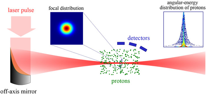


Set citation alerts for the article
Please enter your email address

© Copyright 2018-2021 | Chinese Laser Press. All Rights Reserved 沪ICP备15018463号-20