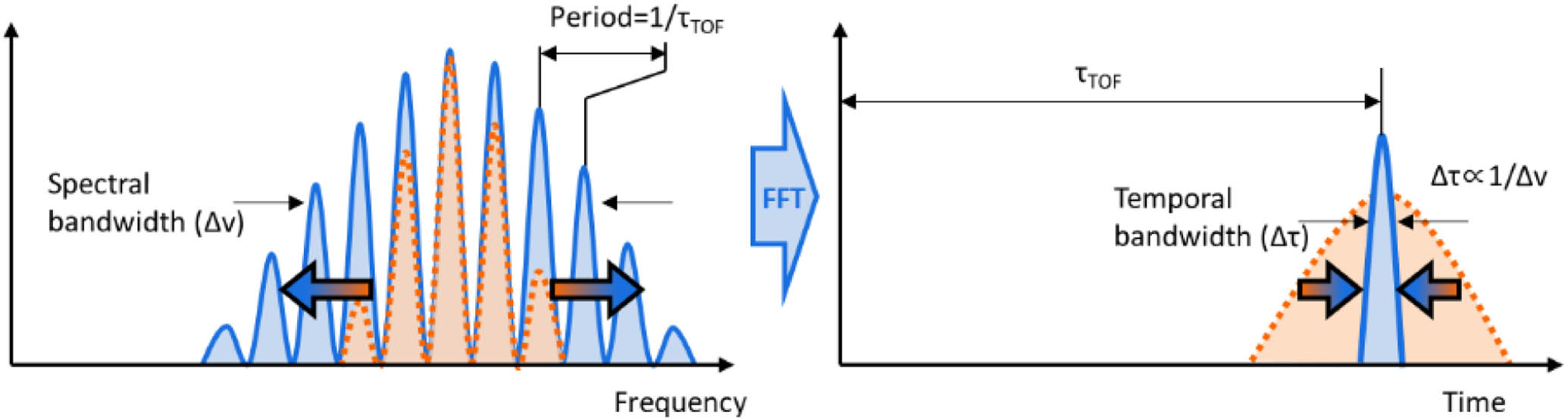
Fig. 1. Relationship between the spectral bandwidth and temporal bandwidth (or dimensional resolution) of the light source in spectral domain interferometry. Blue curves denote broadband light sources and orange dashed curves denote narrowband light sources. As the optical spectrum has larger spectral bandwidth, the converted time domain signal has narrower temporal bandwidth, resulting in high-resolution dimensional metrology. Δv, spectral bandwidth; and Δτ, temporal bandwidth.

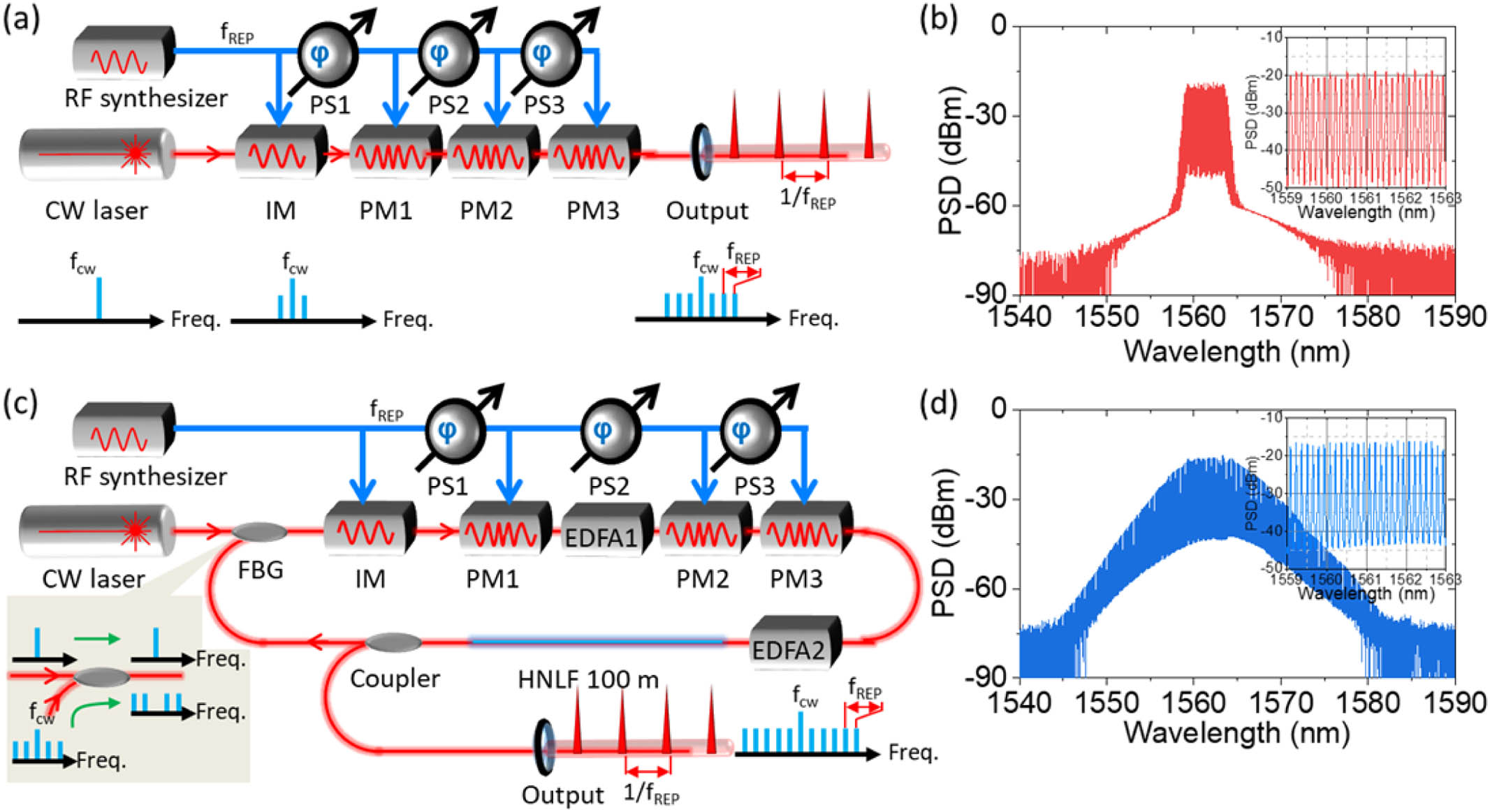
Fig. 2. Broadband EO comb generation. (a) Typical EO comb generation scheme. (b) Generated EO comb from the scheme shown in (a). Inset shows a zoomed-in view. (c) Proposed method of EO comb generation with the optically recirculating loop. (d) Generated EO comb from the scheme in (c). Inset shows a zoomed-in view on a scale identical to that in the inset of (b).

Fig. 3. Optical characterization of the EO comb. (a) Spectral evolution of the EO comb. (b) Long-term stability of the optical spectrum with power amplification of 450 mW. The upper section shows a zoomed-in view of 1560–1565 nm. The red line on the mid-section is the sech2 curve fitting line (see Fig. 8 for an extended view). (c) Pulse duration measurement by the interferometric autocorrelator for power amplification of 450 mW. The filtered autocorrelation signal was fitted to a sech2 curve. (d) Intensity autocorrelation signal for power amplification of 180 mW and 450 mW. The yellow line shows the intensity autocorrelation signal for the single-path EO comb.

Fig. 4. RF characteristics of the EO comb. (a) RF spectrum near the repetition rate with a resolution bandwidth (RBW) and video bandwidth (VBW) of 30 kHz. (b) Repetition rate fluctuation over 10 min. (c) Frequency stability of the repetition rate in terms of the Allan deviation.

Fig. 5. EO-comb-based high-precision distance measurement. (a) Experimental setup of the EO-comb-based spectral interferometer. CL, collimating lens; and M, mirror. (b) Typical spectral interference pattern measured by the spectrometer. (c) Time-dependent variation of the measured distance over 10 s and corresponding histogram. The yellow line in the section on the left shows the 100-point moving-average line. The red line in the section on the right shows the line fitted to a normal distribution. (d) Power spectral density of the measured distance from 0.1 Hz to 1.5 kHz. (e) Measurement repeatability in terms of the Allan deviation. The gray dashed line denotes the white-noise-limit fitted line. The green dashed line and yellow dashed line are the numerical simulation results for the intensity-fluctuation-induced measurement repeatability. (f) Measurement linearity test results with the laser displacement interferometer over 1.6 mm in 0.2 mm steps.

Fig. 6. Comparison of the measurement capabilities with state-of-the-art absolute distance measurement methods. The horizontal axis shows the update rate of the measurement and the vertical axis shows the repeatability without averaging. The yellow diagonal dashed line shows the white-noise-limited precision at an averaging time of 1 s. (See Appendix D.)

Fig. 7. Frequency variation of the seed laser induced measurement error. (a) Frequency variation of the seed laser induced measurement error for 1 mm, 100 mm, and 10 m, typical FFT peak detection error and measurement repeatability. (b) Refractive index change induced measurement error for 1 mm, 100 mm, and 10 m.

Fig. 8. Extended view of Fig. 3(b) for the optical spectrum fitted to a sech2 curve. Curve fitting results of the measured spectrum on (a) a log scale and (b) a linear scale.

Fig. 9. Pulse compression for a single path. The pulse durations were measured and found to be 9.5 ps, 1.1 ps, and 2.4 ps for no pulse compression, SMF 300 m, and SMF 500 m, respectively.

Fig. 10. Comparison of numerical simulation and experimental results for measurement repeatability. Thin lines denote the numerical simulation results and thick lines denote the experimental results.