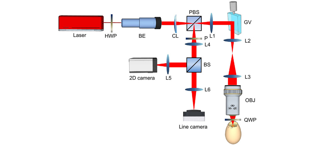
Fig. 1. Schematic diagram of laser speckle autocorrelation imaging system. HWP, half-wave plate; BE, beam expander (3×); CL, cylindrical lens; PBS, polarizing beam splitter; GV, 1-D galvo mirror; OBJ, objective lens; QWP, quarter-wave plate; TS, translational stage; P, polarizer. BS, beam splitter (50/50). The focal length of CL is 50 mm. Focal lengths of lenses L1, L2, L3, L4, L5 and L6 are 50, 50, 100, 40, 75 and 100 mm, respectively. The numerical aperture (NA) of the objective lens (4×) is 0.1.

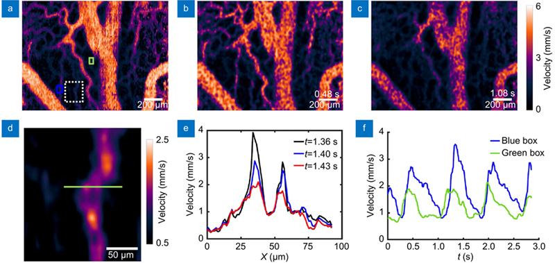
Fig. 2. Blood flow velocity images obtained from chicken embryo No. 1 using LS-LSAI. (a) An averaged blood flow velocity map over the entire image stack. (b) An instantaneous blood flow image at the time point 0.48 s, when the flow velocity reached the maximum. (c) An instantaneous blood flow image at the time point 1.08 s, when the flow velocity reached the minimum. (d) A magnified view of the white dashed boxed region in (a). (e) Cross-sectional flow velocity profiles taken along the green line in (d) at various time points. (f) The time courses of spatially averaged blood flow over the regions indicated by the blue and green squares in (a).

Fig. 3. LS-LSAI dynamic range and FOV. (a) A blood flow velocity image of a chicken embryo (No. 2) scanned at 200 fps for a standard FOV. (b) The comparison of time courses of the blood flow in the same regions [enclosed by the blue box in (a)]. Blue and green curves were related to the acquisition frame rate of 200 fps and 400 fps, respectively. (c) A time-averaged blood flow velocity image of another chicken embryo (No. 3) scanned at 200 fps. (d) The measured intensity temporal autocorrelation function (black circles), which was spatially averaged over a sampling region enclosed by the green box in (c) and fitted curves (solid lines) with models with different n. (e) The measured intensity temporal autocorrelation function at two different time points (circles), and their corresponding fitted curves (lines) with a model parameter n = 1. (f) The time course of the blood flow velocity for the same sampling region.

Fig. 4. Morphological information from the β map. (a) An averaged β map obtained from a chick embryo (No. 4). (b) The contrast-enhanced version of (a). (c) A wide-field color image of the vasculature in the same FOV with white light illumination.

Fig. 5. Comparison of LS-LSAI and LS-LSCI. The averaged velocity images (a) obtained with LS-LSCI with the exposure time of 24 ms and (b) LS-LSAI with the exposure time of 0.04 ms. (c) The flow velocity profiles taken along the white line in (a) and (b). (d) The spatially averaged blood flow velocity and standard deviation at the positions indicated by the white regions of interest (ROI) in (a) and (b).

Fig. 6. LS-LSAI/SI-LSCI image fusion. (a) A LS-LSAI flow image. (b) The speckle contrast image of the same FOV acquired by SI-LSCI. (c) The normalized version of (b) with the β map from LS-LSAI. (d) A big vessel mask derived from (a). (e) and (f) Merged flow images at t=1 s and t=1.47 s, respectively. The same color map and color bar apply to (a), (e), and (f).