Laser speckle imaging has been widely used for in-vivo visualization of blood perfusion in biological tissues. However, existing laser speckle imaging techniques suffer from limited quantification accuracy and spatial resolution. Here we report a novel design and implementation of a powerful laser speckle imaging platform to solve the two critical limitations. The core technique of our platform is a combination of line scan confocal microscopy with laser speckle autocorrelation imaging, which is termed Line Scan Laser Speckle Autocorrelation Imaging (LS-LSAI). The technical advantages of LS-LSAI include high spatial resolution (~4.4 μm) for visualizing and quantifying blood flow in microvessels, as well as video-rate imaging speed for tracing dynamic flow.
Introduction
Microcirculation consists of the smallest blood vessels in the vascular network, where the interaction between blood and tissue creates an environment necessary for cell and tissue survival1. Dynamic blood flow velocity imaging of microcirculation may shine a new light on possible pathophysiological mechanisms of various diseases and is therefore of importance for diagnosis, therapy planning, and monitoring of cancer, vascular rheumatoid, and other diseases2, 3. Optical techniques based on the statistics of laser speckles, including laser speckle contrast imaging4, 5 and laser speckle autocorrelation imaging6, are the most common methods for non-invasive, in vivo blood flow measurements in tissue microvasculature. However, it is very difficult for these established methods to meet the requirements in microcirculation imaging. Besides the high spatial resolution for visualizing capillaries, a high temporal resolution is also needed to capture the time-dependent changes of blood flow velocity. Microcirculatory blood flow is dynamic on various time scales. Previous studies have shown that blood flow in human skin capillaries has a pulsating nature (~1 Hz)7. Arterioles change their tone and lumen size constantly, contracting and relaxing on an average frequency of 0.1 Hz. The oscillatory nature of cutaneous perfusion is caused by the functional activity of various regulatory mechanisms and has the potential to become an important biomarker for telemedicine8. In neuroscience, the regulatory mechanisms of cerebral microcirculation have attracted a great deal of interest. The hemodynamic processes, in terms of vasoactive segments, capillary recruitment, blood cell velocity and flow, underlying adaptive changes in cerebral microcirculation remain to be determined.
Laser speckle contrast imaging (LSCI) uses the spatial or temporal blurring of the speckles to quantify blood flow. It has been widely used to monitor blood flow changes in ophthalmology9-12, dermatology13, 14, and neuroscience15-21. There has been some recent progress on the theoretical models, instrumentation, and biomedical applications of LSCI22-26. Duncan and Kirkpatrick27 explored the impact of various analytic models for relating speckle contrast to scatterer motion. Parthasarathy et. al.18, 28 developed a Multi-Exposure Speckle Imaging instrument and a new speckle model for better quantifying flows in the presence of static scatterers. The technique was found to improve estimates of relative blood flow changes. Parthasarathy et. al.29 and Richards et. al.30 showed that LSCI could obtain blood flow images in humans in real-time during neurosurgery and had the potential to be a valuable intraoperative monitoring tool for a variety of neurosurgical procedures. Laser Speckle Autocorrelation Imaging (LSAI), on the other hand, finds the light intensity auto-correlation to quantify the blood flow. Postnov et. al.6 demonstrated that the wide-field laser speckle intensity temporal autocorrelation function could be obtained using a camera of high frame rate. The measured field autocorrelation function was used to choose the appropriate model for quantifying the blood flow. Recently, it was reported that microvascular imaging with LSAI is better than LSCI under the same condition because of its higher sensitivity to slow flows31.
Both LSCI and LSAI techniques have been conventionally implemented on wide-field optical imaging platforms, where a sample surface is uniformly illuminated with a laser beam and a camera is used to capture the two-dimensional speckle patterns. It is well known in the light microscopy society that wide-field imaging methods suffer from deteriorated spatial resolution and contrast when the sample is optically thick. Similarly in laser speckle imaging, out-of-focus and multiply scattered light in the sample makes it difficult to achieve high-resolution flow mapping and consistent flow quantification. To improve the spatial resolution and flow quantification, it is necessary to introduce focused illumination and confocal detection as implemented in a confocal microscope. Nonetheless, the focused illumination needs to be scanned across the sample surface and the image acquisition speed usually is slowed down significantly, especially in case of point-to-point scanning. Recently, the line-scanning strategy has been adopted in fluorescence microscopy32-34 as well as optical coherence tomography35 to achieve the optimal compromise between the imaging speed and multiple scattering suppression. The combination of line-scanning image acquisition and speckle contrast, however, has yet accomplished the desired temporal resolution for dynamic flow imaging36.
Here we report a Line Scan Laser Speckle Autocorrelation Imaging (LS-LSAI) technique to overcome the technical shortcomings of existing laser speckle imaging methods for label-free microcirculation imaging. LS-LSAI is implemented on top of a line scan confocal microscope for suppressing the out-of-focus and multiply scattered light. Its sample scanning and image acquisition processes are so designed to enable a very short line exposure time (tens of microseconds), which leads to a high speckle acquisition speed of more than 200 fps. Such high acquisition speed makes it possible for LS-LSAI to derive the flow information from temporal speckle autocorrelation, and the resultant flow velocity maps can be created at a video rate. Animal imaging experiments have been conducted to validate the spatial resolution, temporal resolution, as well as flow quantification robustness of this novel approach.
LS-LSAI method
Imaging system design and implementation
The experimental setup for LS-LSAI is essentially a confocal laser scanning optical microscope. Nonetheless, there are several key technical features different from conventional confocal microscopy, which are crucial for fast laser speckle imaging. First of all, the laser source in the LS-LSAI system is a so-called single-frequency laser that has a very long coherence length and good spatial coherence. The coherence properties of the laser are essential for achieving the best speckle contrast. Secondly, a cylindrical is utilized to condense the laser beam in one dimensional and form an illumination line on the sample.
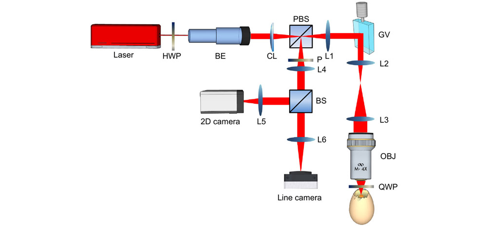
The schematic of the imaging system is illustrated in Fig. 1. A 640 nm/25 mW solid-state single-frequency laser with a coherence length greater than 300 m (RCL-025-640-S, CrystaLaser) is used as a light source. As the laser output is linearly polarized, a half-wave plate (HWP) is used to rotate the polarization direction so that most of the laser beam can pass through the polarizing beam-splitter (PBS). A beam expander, enclosed in the dashed black box, is used to expand the collimated laser beam so that a large illumination area can be covered. A cylindrical lens (ACY254-050-A, Thorlabs) is used to condense the light in one dimension and generate an illumination line. A 1-D galvo mirror (GVS011, Thorlabs) is employed to scan the illumination line across the sample surface. The back-scattered photons from the sample are collected by the objective lens, de-scanned, and travel back along the detection light path. A quarter-wave plate (QWP) manipulates the polarization of the incident and back-scattered light so that the latter is mostly reflected by the PBS. A 50/50 beam splitter is then used to direct the back scattered photons towards a 12-bit ultra-fast line camera (Basler-raL4096-80 km) for the line scan imaging modes and a 2-D monochrome camera (UI-3240CP, IDS) for the wide-field image acquisition modes (with the cylindrical lens removed). To minimize the specular reflection from optical surfaces, a linear polarizer is placed in front of the BS and its orientation is set perpendicular to that of the illumination beam polarization. For system control, we have designed a customized LabVIEW program and utilized a NI PCI-6115 data acquisition card and a NI PCIe-1433 image acquisition board to synchronize the galvo mirror and the camera.
Figure 1.Schematic diagram of laser speckle autocorrelation imaging system. HWP, half-wave plate; BE, beam expander (3×); CL, cylindrical lens; PBS, polarizing beam splitter; GV, 1-D galvo mirror; OBJ, objective lens; QWP, quarter-wave plate; TS, translational stage; P, polarizer. BS, beam splitter (50/50). The focal length of CL is 50 mm. Focal lengths of lenses L1, L2, L3, L4, L5 and L6 are 50, 50, 100, 40, 75 and 100 mm, respectively. The numerical aperture (NA) of the objective lens (4×) is 0.1.
The interference between the wavelets coming from scatterers inside the sample results in speckle patterns picked up by the line camera. The speckle contrast tends to decrease with an increasing exposure time. Therefore, the smallest possible exposure time is desirable to maximize the speckle contrast. A practical limitation of the camera exposure time is the number of photons collected by the sensing elements, which determines the shot noise limited image quality. In a conventional LSAI system with surface illumination, a high illumination power is needed to maintain a short exposure time. In contrast, the line scan setup allows a significantly reduced illumination power as the laser beam is confined to a much smaller sample area.
The raw speckle images are processed to create flow images and videos using established theoretical models, which are based on the temporal statistics of the speckle pattern. From the speckle intensity, we derive the intensity temporal autocorrelation function at any time t using the following formula
where Iis the speckle intensity, is the time lag, and is the width of a time window for averaging. As the raw speckle patterns are recorded frame by frame at a preset repetition rate, the time averaging operations are typically performed over a time window of 5–30 consecutive speckle frames. This time t could be shifted at various time steps within the image stack to evaluate the temporal evolution of . The behavior of is associated with the instantaneous and local motion of scatters. According to established theoretical models, the intensity autocorrelation function is related to a characteristic parameter, the correlation time of the scatterers by
where is a parameter that accounts for the reduction in the speckle contrast due to various reasons and n takes values of 0.5, 1, or 2 depending on the light scattering regime (single or multiple) and particle motion type (ordered or unordered). It has been experimentally determined that is the optimal choice for LS-LSAI. Using Eq. (2), it is straightforward to retrieve the best-fitted parameters and pixel by pixel from the speckle image sequence for any time t. By shifting the time t at 10 ms (2 frames) a step in the raw speckle image stack, a flow velocity video with a frame rate of 100 fps could be readily created.
Our microcirculation imaging results suggest that the parameter is related to the characteristics of moving scatterers in different anatomical structures and could be used to delineate the tissue morphology. The correlation time can be converted to the flow velocity using the following equation27
where is the characteristic width of the Airy function, which describes the best-focused spot of light that passes through a focusing lens. It is limited by the diffraction of light and its value depends on the wavelength of light and the numerical aperture of the lens.
Our current setup also allows us to perform line scan laser speckle contrast imaging (LS-LSCI), for which a long line exposure time is used. In addition, the 2-D camera enables conventional surface illumination (SI-LSCI). Both LS-LSCI and SI-LSCI rely on the speckle contrast, which is related to the correlation time by28
where K is the speckle contrast, σ is the standard deviation of the speckle intensity, is the mean intensity, and T is the exposure time of the camera. In this study, both the mean and standard deviation were evaluated spatially by the use of a sample window. Typically a 7×7 pixel window was used for SI-LSCI while in LS-LSCI the window size was 7 pixels along the camera line13, 22. It should be noted that the parameter may vary from one imaging mode to another.
Live animal imaging
Chick embryos have been widely employed as a small animal model for cardiovascular research. In this work, a series of imaging experiments have been conducted with day 3 chick embryonic samples to evaluate the proposed laser speckle imaging methods in visualizing blood flow in microvessels. The samples were typically scanned repeatedly at a frame rate of 200 frames per second (fps). The line camera was operated at 20 kHz and with an exposure time of 0.04 ms unless stated otherwise. Consequently, it took 5 ms to acquire one speckle image frame consisting of 100 lines. The optics and scanning mechanism were so configured that the typical field of view (FOV) was 1.56 mm in width (along the illumination line) and 1.17 mm in height (along the line scanning direction). Usually, an image stack of 600 frames was obtained in each image acquisition process to cover a few cardiac cycles.
The raw speckle image stacks acquired from samples were processed to create maps of two dynamic scattering parameters and . The speckle correlation time at any time and any location was then translated to an instantaneous, local blood velocity. The parameter was a correction factor that, according to literature, depended on the geometry and alignment of the laser beam in the light scattering setup. However, we have found that maps carried very useful information for both morphological and functional imaging.
Fertilized chicken eggs were purchased from a local poultry farm (Lian Wah Hang Farm PTE LTD, Singapore). The eggs were incubated at 75% humidity and 38.5 °C. On embryonic day 3 (Hamburger-Hamilton stage 18), blunt forceps were used to puncture a hole on the top of the egg where the air pocket was located. The shell membranes were removed with sharp forceps to directly see the whole chick embryo. The egg was then placed on the sample holder and ready for imaging. All the experiments conducted have been reviewed and approved by the Institutional Animal Care and Use Committee (IACUC) of the National University of Singapore.
Results
Spatial and temporal resolutions of LS-LSAI
The advantageous performance of LS-LSAI in terms of spatial and temporal resolutions was verified with imaging experiments on dynamic blood flow in chick embryo microvasculature. Shown in Fig. 2(a) is an example LS-LSAI image obtained from a day 3 chick embryo (sample No. 1) with a line exposure time of 0.04 ms and a frame rate of 200 fps. It maps the time-averaged (over the entire image stack) blood velocity in a complex network of blood vessels of various sizes. Two representative instantaneous flow velocity maps are provided in Fig. 2(b) and 2(c), showing time-dependent flow changes. They were excerpted from a flow velocity image sequence (Supplementary Vidoe S1), which was rendered at 100 fps. The magnified view of the white dashed box in Fig. 2(a) shows two microvessels very close to each other and entangled in the space [Fig. 2(d)]. Plotted in Fig. 2(e) are cross-sectional flow velocity profiles at various time points. They were taken along the green line in Fig. 2(d). These two microvessels had a center-to-center distance of around 16 µm. Their diameters were estimated to be around 10 µm. Shown in Fig. 2(f) are time courses of spatially averaged flow velocity in the green and blue boxes, which were sampled at a time interval of 10 ms. They were different not only in the pulse amplitude but also in terms of the cardiac phase and detailed pulse shape. LS-LSAI was capable of providing excellent time and spatial resolutions simultaneously to capture detailed dynamic flow information from the microvasculature in a live animal model.
Figure 2.Blood flow velocity images obtained from chicken embryo No. 1 using LS-LSAI. (a) An averaged blood flow velocity map over the entire image stack. (b) An instantaneous blood flow image at the time point 0.48 s, when the flow velocity reached the maximum. (c) An instantaneous blood flow image at the time point 1.08 s, when the flow velocity reached the minimum. (d) A magnified view of the white dashed boxed region in (a). (e) Cross-sectional flow velocity profiles taken along the green line in (d) at various time points. (f) The time courses of spatially averaged blood flow over the regions indicated by the blue and green squares in (a).
The typical speckle acquisition speed of the LS-LSAI system was set to 200 fps and each speckle frame consisted of 100 lines. The frame period limits the maximal flow velocity that could be quantified accurately, which is estimated by
here is the frame period, and is the lower bound of the ratio used in data analysis. In this study, we set to around 0.01 according to the noise level of the LS-LSAI instrument. The configuration parameters ms and led to a maximal flow velocity of roughly 4.6 mm/s. While such an upper limit was fine for the flow in microvessels, it became problematic for mapping blood flow in relatively big vessels.
In situations where a larger dynamic range was necessary, the LS-LSAI system could be configured to scan the sample with a reduced FOV and an increased frame rate. Such flexibility was demonstrated with imaging results from chick embryonic sample No. 2. The sample was firstly scanned at 200 fps and an LS-LSAI image stack of 286 frames was obtained. All the frames in the stack were utilized to create a time-averaged blood flow map [Fig. 3(a)]. A smaller field of view (1.56 mm × 58.5 μm, as indicated by the white dashed box) was then selected and scanned at 400 fps while each frame consisted of 50 lines. The resultant blood flow velocity movie (Supplementary Video S2) consisted of 586 frames. In both cases, the line exposure time was 0.04 ms. However, it took only 2.5 ms to acquire one speckle image in the latter case. The waveforms of the blood flow in a relatively large vessel are compared in Fig. 3(c). The blue and green curves are the time courses of the blood flow in the blue square marked region in Fig. 3(a) but are related to the frame rate of 200 fps and 400 fps, respectively. It is noticeable that the frequency of the green signal is lower than that of the blue signal. This is due to the reduced heart rate of the embryo after the initial image acquisition procedure. For the typical 200 fps configuration, the flow velocity peak was suppressed and capped around 4.6 mm/s. With the speckle acquisition speed increased to 400 fps, however, the flow measurement range was extended to over 9 mm/s and the pulsatile blood flow in relatively big vessels could be quantified more accurately.
Figure 3.LS-LSAI dynamic range and FOV. (a) A blood flow velocity image of a chicken embryo (No. 2) scanned at 200 fps for a standard FOV. (b) The comparison of time courses of the blood flow in the same regions [enclosed by the blue box in (a)]. Blue and green curves were related to the acquisition frame rate of 200 fps and 400 fps, respectively. (c) A time-averaged blood flow velocity image of another chicken embryo (No. 3) scanned at 200 fps. (d) The measured intensity temporal autocorrelation function (black circles), which was spatially averaged over a sampling region enclosed by the green box in (c) and fitted curves (solid lines) with models with different n. (e) The measured intensity temporal autocorrelation function at two different time points (circles), and their corresponding fitted curves (lines) with a model parameter n = 1. (f) The time course of the blood flow velocity for the same sampling region.
Single-line LS-LSAI was attempted with chick embryo No. 3. After capturing LS-LSAI images at 200 fps, a horizontal line across a big vessel was selected on the averaged blood flow velocity image [see Fig. 3(c)]. Line speckle patterns were acquired continuously at the same position at the line exposure time of 0.04 ms and a repetition rate of 20 kHz. The intensity temporal autocorrelation function was evaluated for each pixel and then fitted to theoretical models [Eq. (2)] of different values for the parameter n. Fig. 3(d) shows an example of the measured and the three fits (n = 0.5, 1, 2) at the position indicated by the green box in Fig. 3(c). Comparing the R2 values of the three fits, we found that was consistently the optimal choice. Therefore, this model was chosen to process all other LS-LSAI data acquired in this work to retrieve the correlation time. Shown in Fig. 3(e) are two examples of the intensity temporal autocorrelation functions (circles) measured at the green box and their corresponding fits (lines). They were acquired at 0 s (red) and 0.35 s (blue) and the fitted correlation times were 396 µs and 2.65 ms, respectively. The complete time course of the blood flow velocity at the same location is shown in Fig. 3(f). The peak velocity in this big vessel (~0.2 mm in diameter) was found to exceed 25 mm/s, which was far greater than the dynamic range for a typical scanning configuration.
β mapping and morphological imaging
We have found in our experiments that the parameter is robustly associated with the tissue type. Shown in Fig. 4(a) is the time-averaged map obtained from chick embryo No. 4. It was observed that was usually very small (smaller than 0.1) in the non-vessel regions, while its value became significantly higher in the vessels. Surprisingly, smaller vessels were generally associated with higher values than big ones. Fig. 4(b) is the contrast-enhanced version of Fig. 4(a), which better delineates the vascular network. One can find a striking similarity in terms of morphological features between Fig. 4(b) and Fig. 4(c), which was obtained from the same sample area using a color CCD camera and white light illumination. On the other hand, the image quality afforded by mapping was much better than that of the wide-field color imaging method.
Figure 4.Morphological information from the β map. (a) An averaged β map obtained from a chick embryo (No. 4). (b) The contrast-enhanced version of (a). (c) A wide-field color image of the vasculature in the same FOV with white light illumination.
The main moving scatterers in tissue that contributed significantly to dynamic light scattering were red blood cells. Therefore, the parameter tended to be small in non-vessel regions where static reflection dominated the detected light intensity. For big vessels, the correlation time might not be significantly greater than the line exposure time and there could be nontrivial speckle blurring. This could be a factor that led to a reduced in comparison with small vessels.
The morphological imaging capability of mapping provided an additional benefit in functional flow imaging. In non-vessel regions where was small and dynamically scattered light intensity was weak, the fitted correlation time and flow velocity might not make sense as they could be overwhelmed by measurement noises. In addition, the applicability of those simple theoretical models became questionable. Vascular structures retrieved from maps made it possible to restrict flow velocity estimation to the vessel regions. In this way, the generated flow maps could afford much-reduced background noise.
Multimodality cross-validation and comparison
Our current setup could also perform line scan laser speckle contrast imaging (LS-LSCI) by choosing a line exposure time suitable for this contrast mechanism36. Compared to LS-LSAI, LS-LSCI generally required a significantly longer line exposure time to measure flow-induced speckle contrast reduction. Both LS-LSCI and LS-LSAI images were obtained from chick embryo No. 4 for cross-validation and performance comparison.
Figure 5(a) shows the blood flow velocity image obtained by using LS-LSCI with a line exposure time of 24 ms and by averaging over 30 frames. The LS-LSCI acquisition time was much longer than the chick embryo cardiac period and lacked the dynamic imaging capability as LS-LSAI did. To make a proper comparison in other aspects, a time-averaged blood flow velocity image [Fig. 5(b)] of the same sample area was obtained in the LS-LSAI mode with a line exposure time of 0.04 ms and a scanning rate of 200 fps. Figure 5(c) shows the blood flow velocity profiles taken along the white lines in Fig. 5(a) and 5(b), respectively. The spatially averaged blood flow velocity and standard deviation at three regions of interest (ROI) indicated in Fig. 5(a) and 5(b) are displayed in Fig. 5(d). It was observed that the image quality, in terms of spatial resolution and noise level, was significantly improved with LS-LSAI. The two flow profiles in Fig. 5(c) were fairly close to each other, indicating that both line scan based imaging modalities were compatible in terms of flow quantification. However, the LS-LSCI profile (blue line) was noisier [see Fig. 5(d)] and the radial distribution tended to shrink in comparison with the LS-LSAI profile (red line). The shrinkage was caused by spatial sampling in LS-LSCI for evaluating the speckle contrast. There were always variations in the mean intensity across the vessel boundaries due to higher light attenuation by blood, which led to overestimated spatial speckle contrasts and consequently underestimated blood flow velocities in regions close to the vessel walls. The LS-LSAI method, by contrast, processed the temporal speckle data pixel by pixel and there was no loss of spatial information.
Figure 5.Comparison of LS-LSAI and LS-LSCI. The averaged velocity images (a) obtained with LS-LSCI with the exposure time of 24 ms and (b) LS-LSAI with the exposure time of 0.04 ms. (c) The flow velocity profiles taken along the white line in (a) and (b). (d) The spatially averaged blood flow velocity and standard deviation at the positions indicated by the white regions of interest (ROI) in (a) and (b).
It is worthy of note that the theoretical model (Eq. (4)) used to translate the LS-LSCI raw data to flow maps also included the parameter . However, such information was not available from the LS-LSCI measurement. The map retrieved from LS-LSAI images [related to Fig. 5(b)] was involved in interpreting the spatial speckle data. Without such a priori information, the flow velocity would have been significantly overestimated by simply assuming .
Fused LS-LSAI/SI-LSCI images
A 2D camera has been included in our imaging set-up to enable the conventional surface illumination laser speckle imaging (SI-LSCI) mode, which augments line scan confocal detection based imaging modes. A computational procedure was devised to further enhance the dynamic range of flow velocity measurement by combining the information from both SI-LSCI and LS-LSAI images.
As shown in Fig. 6(a), which is an LSAI image obtained from chick embryo No. 5, the blood flow velocities in big vessels with a diameter greater than 100 μm appeared to have reached the maximum. No dynamic change could be seen in the corresponding image stack. To improve flow mapping in big vessels without compromising the capability of small vessel imaging, the following steps were followed to create fused SI-LSCI/LS-LSAI images.
Figure 6.LS-LSAI/SI-LSCI image fusion. (a) A LS-LSAI flow image. (b) The speckle contrast image of the same FOV acquired by SI-LSCI. (c) The normalized version of (b) with the β map from LS-LSAI. (d) A big vessel mask derived from (a). (e) and (f) Merged flow images at t=1 s and t=1.47 s, respectively. The same color map and color bar apply to (a), (e), and (f).
First of all, an SI-LSCI image stack was captured for the same field of view at 30 fps and with an exposure time of 2 ms. Fig. 6(b) shows a representative frame of the spatially evaluated speckle contrast (K). As expected, the speckle contrast in big vessels was significantly reduced due to faster flow in them and cardiac fluctuations could be traced from frame to frame. However, converting this K map to flow velocity was difficult since no information about was available from the SI-LSCI measurement. While maps had been generated from LS-LSAI, they might lead to model errors due to the big difference in the optical sectioning capability between LS-LSAI and SI-LSCI. In this work, we employed a simple empirical model to link the maps of the two imaging modalities. It was found that yielded the flow velocities in big vessels in a range best matching single line LSAI measurements. Fig. 6(c) shows a normalized K map, which was obtained by dividing Fig. 6(b) by the map. Surprisingly, some small vessels missing in Fig. 6(b) became visible after the normalization. However, quantification of blood flow in those small vessels remained inaccurate by direct translation of the normalized K map. It was evident that wide-field laser speckle imaging was fundamentally limited in imaging microcirculation. Therefore, only flow information from big vessels was included in the fused images by the use of a mask [Fig. 6(d)], which was derived from Fig. 6(a) with appropriate image processing procedures performed in ImageJ. In the next step, the K map, , and the mask were combined to create masked SI-LSCI velocity maps. Eventually, the masked SI-LSCI images and original LS-LSAI images were merged by taking the maximal value for each spatial location and time point. Fig. 6(e) and 6(f) are two fused velocity maps at two different time points, when the flow velocities in big vessels reached their maximum (around 20 mm/s) and minimum (around 4 mm/s), respectively. Dynamic blood flow changes in both big and small vessels can be observed in more detail in the fused movie (Supplementary Video S3), which was rendered at 30 fps.
Discussion
We have built a laser speckle imaging system, which can be configured to perform LS-LSAI, LS-LSCI, and SI-LSCI imaging. However, the core technique is LS-LSAI while the other two imaging modes are complementary. Compared with existing laser speckle imaging methods, the advantages of LS-LSAI lie in the combination of confocal detection, fast scanning with line illumination, and temporal correlation based speckle analysis. Processing of temporal speckle data pixel by pixel does not involve spatial sampling and therefore helps preserve the spatial resolution. Moreover, it avoids biased estimation in the speckle contrast caused by inherent spatial variation due to morphological heterogeneity in the tissue. To obtain a meaningful speckle dataset for autocorrelation analysis, however, the acquisition speed needs to be adequately high. Even in microvessels, the blood flow is associated with a correlation time of a few milliseconds. Consequently, a frame rate above a few hundred Hertz is necessary. Such a high speed is enabled by scanning the sample line by line. Confocal detection of backscattered light makes it possible to have a well-defined focal volume, relatively independent of the focal depth and the optical properties of the tissue. While the contribution from multiply scattered light is largely suppressed by confocal detection, a more straightforward and consistent relationship between the local flow velocity and the speckle derived correlation time can be expected.
The typical LS-LSAI acquisition speed of 200 fps used in this study was limited by several factors. First of all, the incident light power on the sample surface was only 11 mW. This was remarkably lower than 200 mW used by Postnov et. al. in their wide-field dynamic laser speckle imaging experiments6. The maximal power that can be safely used for in vivo imaging experiments depends on a lot of factors such as the illumination pattern (e.g., point, line, or area), the scanning area, the scanning speed, and the optical and thermal properties of the tissue sample under investigation. Compared with mouse brain models, chick embryos were more sensitive to the illumination light. We had to maintain a relatively low optical power so that the embryonic samples could survive the experiments. The line camera employed for detecting the backscattered photons was designed for machine vision application. Its readout noise was roughly 30e–, which was much inferior to most scientific cameras for biological research. Consequently, an exposure time of 0.04 ms was almost the minimum value to maintain an acceptable signal to noise ratio. One way towards faster scanning is to replace the line camera with a two-dimensional scientific camera and use the dual-Galvo-mirror configuration33. This may help reduce the exposure time by one order of magnitude and consequently enhance the dynamic range of flow quantification by the same magnitude. In applications where the sample is less sensitive to the incident power, a higher power laser would be a good solution.
The spatial resolution was roughly 4.4 microns along the illumination line (horizontal) and 12 microns along the scanning direction (vertical). The horizontal resolution was limited by the numerical aperture (~0.1) of the objective lens while the vertical resolution was essentially the spacing of illumination lines. A more isotropic and finer spatial resolution could be achieved by decreasing the illumination line scanning step size by, for example, a factor of three. However, the expense would be a reduced field of view. Given the exposure time of the line camera, there was limited room to go beyond 100 lines per frame as that would slow down the frame acquisition speed and lead to a smaller value for the flow velocity upper bound. In principle, a large sample area could be divided into multiple smaller FOVs to perform standard scanning procedures with the current setup. In case that the blood flow in the microvasculature is periodic, the small FOVs can be stitched together nicely once the corresponding image stacks are time aligned in the cardiac phase. Of course, this is a rather time consuming and tedious process. A better alternative would be a higher power laser and/or a lower noise camera. While it is expected that LS-LSAI should be able to provide better depth resolution in comparison with wide-field methods, it is beyond the scope of this study. More experiments need to be conducted to quantitatively validate such an advantage.
The LS-LSCI modality is not limited by the number of lines per frame. As long as the dynamic information is not important for the applications, LS-LSCI could be an alternative way to generate time-averaged flow maps with high spatial resolution in both directions. Nevertheless, it is still desirable to also acquire LS-LSAI for the same FOV albeit with a poor vertical resolution. The map from LS-LSAI is essential for more accurately translating the speckle contrast data to flow velocity maps.
The combination of LS-LSAI and SI-LSCI seems to be a promising direction for simultaneous imaging of blood flows in both big and small vessels. The SI-LSCI modality, however, does not have a well-defined focal volume inside a scattering medium. It is, therefore, nontrivial to utilize the maps for interpreting the wide-field speckle contrast images. Our current model that links the maps of both modalities is purely empirical. The image fusion results presented in this paper should be considered preliminary and qualitative. Further investigation is warranted to explore more rigorous theoretical models.
Conclusion
In summary, we have developed a novel Line Scan Laser Speckle Autocorrelation Imaging (LS-LSAI) method for microcirculation imaging and demonstrated its superior blood flow imaging performance in terms of simultaneously achieved high spatial resolution and high temporal resolution. Besides its functional imaging capability in flow imaging, LS-LSAI is also able to provide high quality morphological images of microvasculature. In addition, LS-LSAI has been implemented on a multimodality platform that supports other laser speckle imaging modes including LS-LSCI and SI-LSCI, for which information from LS-LSAI measurement can help better interpret the speckle data and improve flow quantification. Image fusion procedures have been developed to combine LS-LSAI and SI-LSCI images for significantly enhanced dynamic range in flow measurement.