• Photonics Research
  • Vol. 12, Issue 2, 271 (2024)
Yue Wang1, Dashan Dong1, Wenkai Yang1, Renxi He2, Ming Lei3, and Kebin Shi1、4、5、*
Author Affiliations
  • 1State Key Laboratory for Mesoscopic Physics, Department of Physics, Peking University, Beijing 100871, China
  • 2State Key Laboratory of Membrane Biology, School of Life Sciences, and Biomedical Pioneering Innovation Center (BIOPIC), Peking University, Beijing 100871, China
  • 3School of Physics, Xi’an Jiaotong University, Xi’an 710049, China
  • 4Collaborative Innovation Center of Extreme Optics, Shanxi University, Taiyuan 030006, China
  • 5Peking University Yangtze Delta Institute of Optoelectronics, Nantong 226010, China
  • show less
    DOI: 10.1364/PRJ.500618 Cite this Article Set citation alerts
    Yue Wang, Dashan Dong, Wenkai Yang, Renxi He, Ming Lei, Kebin Shi. Reflective ultrathin light-sheet microscopy with isotropic 3D resolutions[J]. Photonics Research, 2024, 12(2): 271 Copy Citation Text show less
    Design of RTLIS. (a) Diagram of mini-prism reflector that can be used in traditional inverted microscope configurations for light-sheet excitation and detection. (b) Schematic of RTLIS setup. Lens1, f=150 mm; scan lens, EFL=50 mm; tube lens, f=200 mm; lens2, f=200 mm; sCMOS: scientific complementary metal oxide semiconductor.
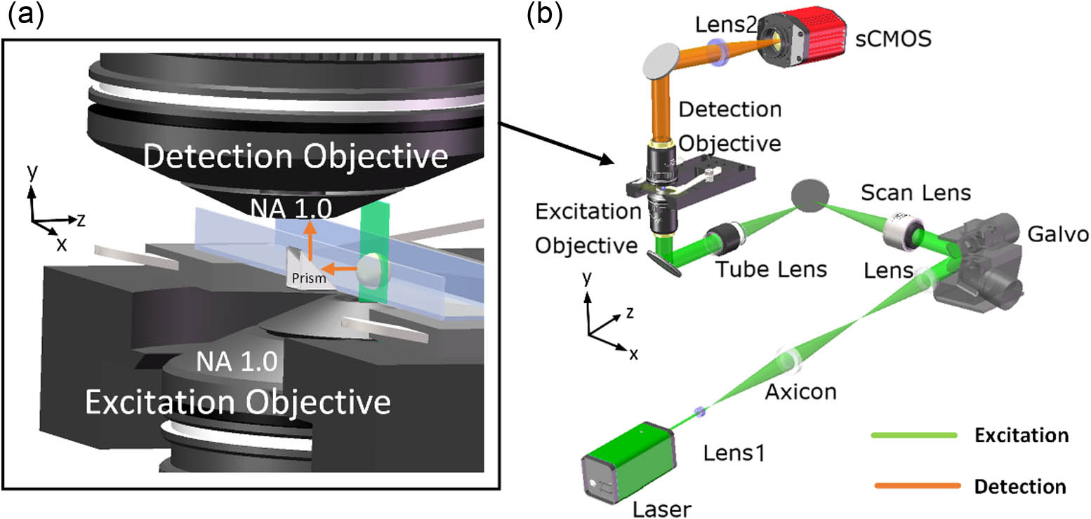
    Fig. 1. Design of RTLIS. (a) Diagram of mini-prism reflector that can be used in traditional inverted microscope configurations for light-sheet excitation and detection. (b) Schematic of RTLIS setup. Lens1, f=150  mm; scan lens, EFL=50  mm; tube lens, f=200  mm; lens2, f=200  mm; sCMOS: scientific complementary metal oxide semiconductor.
    Characterization of the microscope. Representative PSF was obtained by imaging 80 nm fluorescence beads. Projections along XY and XZ are shown in (a) and (b). The Gauss fit curve of the line profiles of the PSF is shown in (c) and (d); the FWHM is 290 nm in X and 310 nm in Z, respectively.
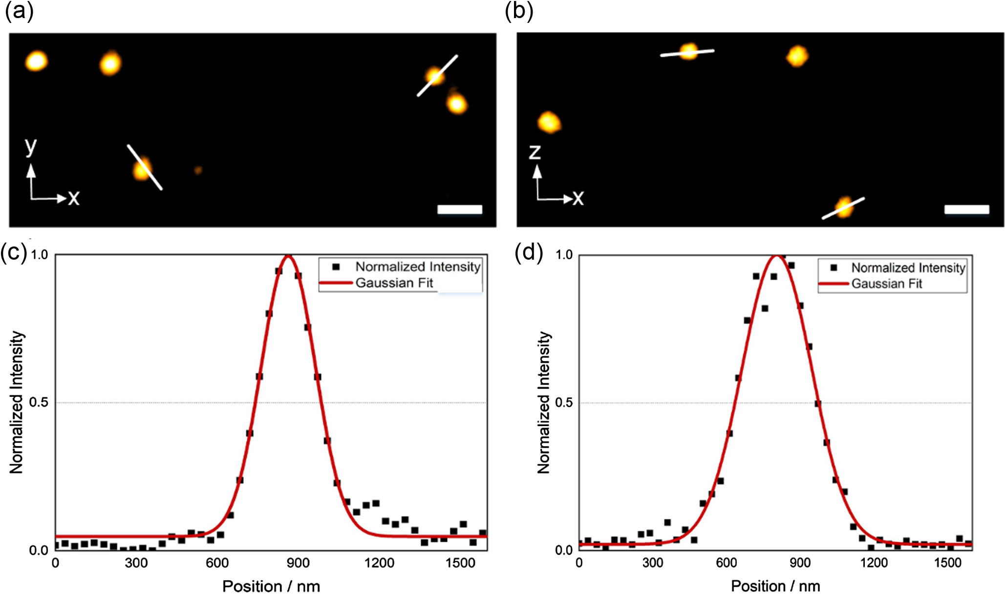
    Fig. 2. Characterization of the microscope. Representative PSF was obtained by imaging 80 nm fluorescence beads. Projections along XY and XZ are shown in (a) and (b). The Gauss fit curve of the line profiles of the PSF is shown in (c) and (d); the FWHM is 290 nm in X and 310 nm in Z, respectively.
    Simulation and experiment results of the characterization of the illumination beam for light-sheet excitation with 561 nm wavelength. (a)–(d) BPM simulation results of the Bessel beam: (a) XZ distribution with NA 1.0 water immersion objective of the Bessel beam; (b)–(d) YZ, XZ, and XY distribution of scanning Bessel light sheet with NA 1.0 water immersion objective, respectively. (e)–(h) Experimental results of the Bessel beam profiles obtained by scanning gold nanoparticle and measuring the scattering signal: (e) XZ distribution with NA 1.0 water immersion objective of the Bessel beam; (f)–(h) YZ, XZ, and XY distribution of scanning Bessel light sheet with NA 1.0 water immersion objective, respectively. (i) The overlap of excitation (green) and detection (blue) PSFs yields the system PSF. (j) PSF of NA 1.0 detection objective in XZ; (k) overall PSF of the light-sheet system. The color scale defines the normalized intensity of the system.
    Fig. 3. Simulation and experiment results of the characterization of the illumination beam for light-sheet excitation with 561 nm wavelength. (a)–(d) BPM simulation results of the Bessel beam: (a) XZ distribution with NA 1.0 water immersion objective of the Bessel beam; (b)–(d) YZ, XZ, and XY distribution of scanning Bessel light sheet with NA 1.0 water immersion objective, respectively. (e)–(h) Experimental results of the Bessel beam profiles obtained by scanning gold nanoparticle and measuring the scattering signal: (e) XZ distribution with NA 1.0 water immersion objective of the Bessel beam; (f)–(h) YZ, XZ, and XY distribution of scanning Bessel light sheet with NA 1.0 water immersion objective, respectively. (i) The overlap of excitation (green) and detection (blue) PSFs yields the system PSF. (j) PSF of NA 1.0 detection objective in XZ; (k) overall PSF of the light-sheet system. The color scale defines the normalized intensity of the system.
    Imaging results of fluorescent microspheres. (a) Imaging result of the 10 μm microspheres; (b) optical sections of 10 μm microspheres at different depths; (c) imaging result of the 2 μm microsphere; (d) imaging result of two fluorescent microspheres in XY-profile with diameters of 10 and 5 μm; (e) imaging result of two fluorescent microspheres in XZ-profile with diameters of 10 and 5 μm; (f) imaging result of two fluorescent microspheres in YZ-profile with diameters of 10 and 5 μm.
    Fig. 4. Imaging results of fluorescent microspheres. (a) Imaging result of the 10 μm microspheres; (b) optical sections of 10 μm microspheres at different depths; (c) imaging result of the 2 μm microsphere; (d) imaging result of two fluorescent microspheres in XY-profile with diameters of 10 and 5 μm; (e) imaging result of two fluorescent microspheres in XZ-profile with diameters of 10 and 5 μm; (f) imaging result of two fluorescent microspheres in YZ-profile with diameters of 10 and 5 μm.
    Imaging results of Drosophila eye’s Rh6 cells. (a) Cross-sectional slices (XY) of the Rh6 cells; (b) cross-sectional slices (XZ) of the Rh6 cells; (c) cross-sectional slices (YZ) of the Rh6 cells.
    Fig. 5. Imaging results of Drosophila eye’s Rh6 cells. (a) Cross-sectional slices (XY) of the Rh6 cells; (b) cross-sectional slices (XZ) of the Rh6 cells; (c) cross-sectional slices (YZ) of the Rh6 cells.
    Design and physical drawings of sample chamber. (a) Open-top glass chamber for biological sample; (b) mini-prism holder; (c) design of the slide; (d) assembled sample holder; (e) photograph of the sample holder with objectives.
    Fig. 6. Design and physical drawings of sample chamber. (a) Open-top glass chamber for biological sample; (b) mini-prism holder; (c) design of the slide; (d) assembled sample holder; (e) photograph of the sample holder with objectives.
    Synchronous timing control diagram of the RTLIS electronics. The sCMOS camera and the galvo signals (X, Z) are done via a National Instruments DAQ, whereas the laser intensity control is realized by the sCMOS camera trigger; the motorized translation stage and the DAQ are both connected to the imaging computer.
    Fig. 7. Synchronous timing control diagram of the RTLIS electronics. The sCMOS camera and the galvo signals (X, Z) are done via a National Instruments DAQ, whereas the laser intensity control is realized by the sCMOS camera trigger; the motorized translation stage and the DAQ are both connected to the imaging computer.
    BPM simulation results of the characterization of the illumination beam and scanned light sheet with 561 nm wavelength. (a)–(d) Results of the Bessel beam with NA 1.0 excitation objective: (a) XZ distribution of the Bessel beam; (b)–(d) YZ, XZ, and XY distribution of scanning Bessel light sheet, respectively. (e)–(h) Results of the Bessel beam with NA 1.4 excitation objective: (e) XZ distribution of the Bessel beam; (f)–(h) YZ, XZ, and XY distribution of scanning Bessel light sheet, respectively. (i)–(l) Results of the Gaussian beam with NA 1.0 excitation objective: (i) XZ distribution of the Gaussian beam; (j)–(l) YZ, XZ, and XY distribution of scanning Gaussian light sheet, respectively. (m)–(p) Results of the Gaussian beam with NA 1.4 excitation objective: (m) XZ of the Gaussian beam; (n)–(p) YZ, XZ, and XY distribution of scanning Gaussian light sheet, respectively. The color scale defines the normalized intensity of the system.
    Fig. 8. BPM simulation results of the characterization of the illumination beam and scanned light sheet with 561 nm wavelength. (a)–(d) Results of the Bessel beam with NA 1.0 excitation objective: (a) XZ distribution of the Bessel beam; (b)–(d) YZ, XZ, and XY distribution of scanning Bessel light sheet, respectively. (e)–(h) Results of the Bessel beam with NA 1.4 excitation objective: (e) XZ distribution of the Bessel beam; (f)–(h) YZ, XZ, and XY distribution of scanning Bessel light sheet, respectively. (i)–(l) Results of the Gaussian beam with NA 1.0 excitation objective: (i) XZ distribution of the Gaussian beam; (j)–(l) YZ, XZ, and XY distribution of scanning Gaussian light sheet, respectively. (m)–(p) Results of the Gaussian beam with NA 1.4 excitation objective: (m) XZ of the Gaussian beam; (n)–(p) YZ, XZ, and XY distribution of scanning Gaussian light sheet, respectively. The color scale defines the normalized intensity of the system.
    Beam profile measurements by scanning gold nanoparticle and detecting the scattering with NA 1.4 excitation oil immersion objectives. (a)–(d) Distribution of the Bessel light sheet: (a) XZ distribution of the Bessel beam; (b)–(d) YZ, XZ, and XY distribution of scanning Bessel light sheet, respectively. (e)–(h) Distribution of the Gaussian light sheet: (e) XZ distribution of the Gaussian beam; (f)–(h) YZ, XZ, and XY distribution of scanning Gaussian light sheet, respectively. The color scale defines the normalized intensity of the system.
    Fig. 9. Beam profile measurements by scanning gold nanoparticle and detecting the scattering with NA 1.4 excitation oil immersion objectives. (a)–(d) Distribution of the Bessel light sheet: (a) XZ distribution of the Bessel beam; (b)–(d) YZ, XZ, and XY distribution of scanning Bessel light sheet, respectively. (e)–(h) Distribution of the Gaussian light sheet: (e) XZ distribution of the Gaussian beam; (f)–(h) YZ, XZ, and XY distribution of scanning Gaussian light sheet, respectively. The color scale defines the normalized intensity of the system.
    Experimental results for resolution calibration using 80 nm fluorescent beads. The first row represents the raw data, while the second row displays the deconvolution results. The scale bar is 500 nm.
    Fig. 10. Experimental results for resolution calibration using 80 nm fluorescent beads. The first row represents the raw data, while the second row displays the deconvolution results. The scale bar is 500 nm.
    Three-dimensional experimental results for 10 and 5 μm fluorescent beads. The first row represents the raw data, while the second row displays the deconvolution results. The scale bar is 7 μm.
    Fig. 11. Three-dimensional experimental results for 10 and 5 μm fluorescent beads. The first row represents the raw data, while the second row displays the deconvolution results. The scale bar is 7 μm.
    Yue Wang, Dashan Dong, Wenkai Yang, Renxi He, Ming Lei, Kebin Shi. Reflective ultrathin light-sheet microscopy with isotropic 3D resolutions[J]. Photonics Research, 2024, 12(2): 271
    Download Citation