
Yang Zhu, Binbin Lu, Zhiyuan Fan, Fuyong Yue, Xiaofei Zang, Alexei V. Balakin, Alexander P. Shkurinov, Yiming Zhu, Songlin Zhuang, "Geometric metasurface for polarization synthesis and multidimensional multiplexing of terahertz converged vortices," Photonics Res. 10, 1517 (2022)
- Photonics Research
- Vol. 10, Issue 6, 1517 (2022)
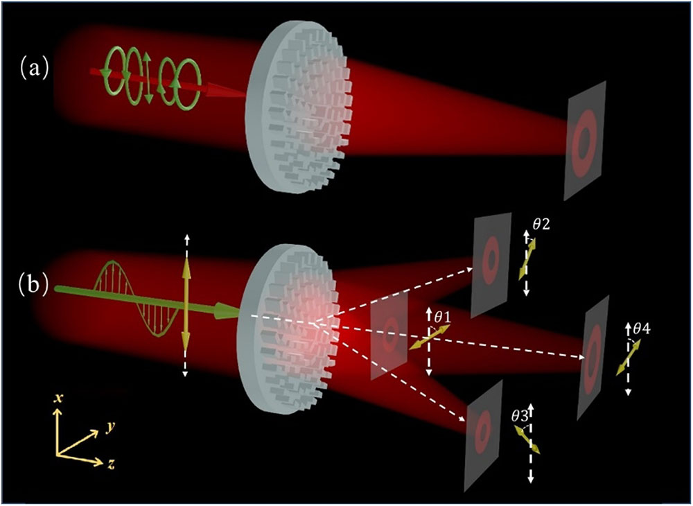
Fig. 1. Schematic of the metasurfaces for polarization-independent vortex and the multiplexing of polarization-rotatable multiple vortices in multiple spatial dimensions. (a) Polarization-independent vortex with identical topological charges generated by a geometric metasurface under illumination of THz waves with arbitrary polarization states. (b) Multiplexing of polarization-rotatable multiple vortices in both transverse and longitudinal directions under illumination of linearly polarized THz waves.
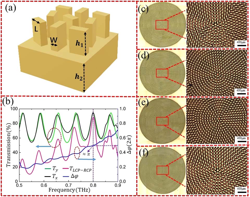
Fig. 2. Design and fabrication of the geometric metasurfaces. (a) Designed geometric metasurface consisting of meta-atoms with identical shapes but different in-plane orientations. (b) Transmission spectra (green and black curves) and phase difference (blue curve) of a meta-atom with the long-axis along the x
Fig. 3. Electric-field intensity and phase distributions of the spin-independent vortices. (a1)–(a5), (c1)–(c5) Simulated and measured electric-field intensity distributions after the designed geometric metasurface under illumination of LCP, LECP, LP, RECP, and RCP THz waves. (b1)–(b5), (d1)–(d5) Simulated and measured phase distributions of the corresponding vortices.
Fig. 4. Electric-field intensity and phase distributions of the multiplexing of two vortices with two orthogonal LP states in the longitudinal direction. (a1)–(b2) Simulated and measured electric-field intensity distributions at z = 4.3 mm z = 7.9 mm x – z
Fig. 5. Electric-field intensity and phase distributions of the multiplexing of four vortices with different LP states in longitudinal and transverse directions. (a1)–(f2) Simulated and measured electric-field intensity and phase distributions at z = 4.3 mm z = 6.3 mm z = 7.9 mm x – z
Fig. 6. Electric-field intensity distributions of a vortex with extended focal length. (a1)–(c2) Simulated and measured electric-field intensity distributions for | E x | 2 | E y | 2 | E x | 2 + | E y | 2 x – z | E x | 2 | E y | 2 | E x | 2 + | E y | 2 x – y
Fig. 7. Schematics of anisotropic meta-atoms without (a) and with (b) a rotation angle.
Fig. 8. Electric-field intensity distributions of spin-independent vortices in the x – z x – z
Fig. 9. Electric-field intensity and phase distributions for the polarization-rotatable vortex (l = 1 x y z = 7.5 mm y z = 7.5 mm | E x | 2 | E y | 2 x – z
Fig. 10. Electric-field intensity and phase distributions of the multiplexing of two vortices with two orthogonal LP states in the transverse direction. (a1)–(a4) Simulated and measured electric-field intensity and phase distributions for | E x | 2 z = 7.5 mm x y z = 7.5 mm | E x | 2 | E y | 2 x – z x – z
Fig. 11. Electric-field intensity and phase distributions of the multiplexing of two vortices with two orthogonal helical states in the longitudinal direction. (a1)–(b2) Simulated and measured electric-field intensity distributions at z = 4.3 mm z = 7.9 mm x – z
Fig. 12. Electric-field intensity and phase distributions of the multiplexing of two vortices with two orthogonal helical states in the transverse direction. (a1)–(b6) Simulated and measured electric-field intensity and phase distributions at z = 7.5 mm x – z
Fig. 13. Electric-field intensity and phase distributions of the multiplexing of three vortices with LP states and CP state. (a1)–(b8) Simulated and measured electric-field intensity and phase distributions at z = 6.3 mm z = 7.9 mm x – z
Fig. 14. Electric-field intensity and phase distributions of the multiplexing of two vortices with two orthogonal CP (a1)–(a6) or LP (b1)–(b6) states in the longitudinal direction. (a1), (a2) Simulated and measured electric-field intensity distributions at z = 4.3 mm z = 7.9 mm x – z z = 4.3 mm z = 7.9 mm x – z
Fig. 15. Phase distributions of a vortex with extended focal length. (a1)–(a6), (b1)–(b6) Simulated and measured phase distributions for x x – y y x – y


Set citation alerts for the article
Please enter your email address

© Copyright 2018-2021 | Chinese Laser Press. All Rights Reserved 沪ICP备15018463号-20