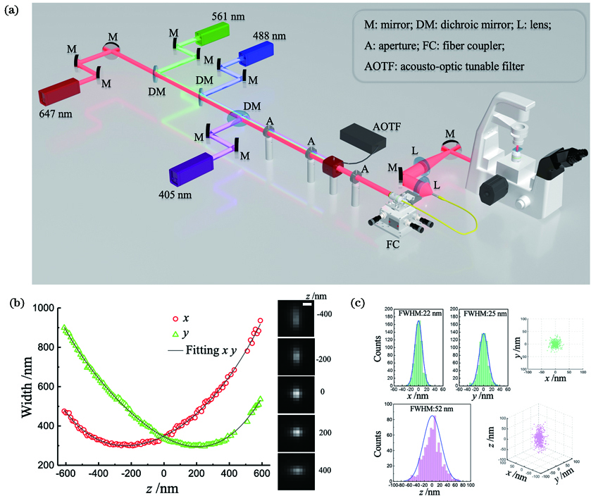
Fig. 1. Principle of 3D-STORM. (a) Optical path diagram of STORM; (b) PSF shape of a fluorophore at various z positions and calibration curves show x and y widths as functions of z (scale bar: 500 nm); (c) 3D localization distribution of single molecule fluorescence

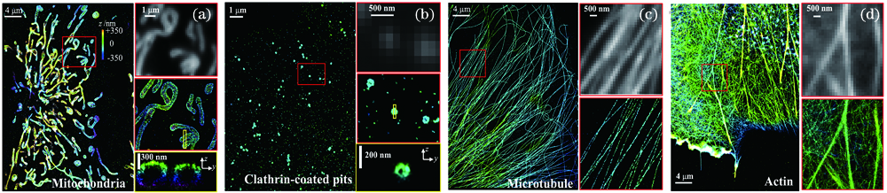
Fig. 2. STORM images of four subcellular structures from Cos7 cell. (a) Mitochondria; (b) clathrin-coated pits; (c) microtubules; (d) microfilaments

Fig. 3. Drift correction of STORM images of tubulin and tropomodulin in x and y directions. (a) STORM images of Cos7 cell microtubule before and after drift correction; (b) STORM images of erythrocyte tropomodulin before and after drift correction; (c) drift correction curves of microtubule images in x and y directions; (d) drift correction curves of erythrocyte tropomodulin in x and y directions

Fig. 4. Images of the same subcellular structures using different sample preparation methods. (a)(b) Images of mitochondria of Cos7 cell labeled with different primary antibodies; (c) images of microtubule of Cos7 cell fixed with methanol; (d) images of microtubule of Cos7 cell fixed with 3% paraformaldehyde+0.1% glutaraldehyde

Fig. 5. Improvement of SMLM lateral resolution based on algorithms or hardware modifications. (a) Improvement of STORM lateral resolution by dual objective fluorescence collection system^[64]; (b) improvement of STORM lateral resolution by particle average algorithm^[65]; (c) improvement of lateral resolution by MINFLUX based on algorithm combined hardware modification^[14]; (d) improvement of lateral resolution by ROSE based on algorithm combined hardware modification ^[66]

Fig. 6. Improvement of SMLM axial resolution based on algorithms or hardware modifications. (a) Improvement of STORM axial resolution by dual objective fluorescence collection system^[64]; (b) improvement of axial resolution by dual objective fluorescence interferometric system ^[71]; (c) improvement of DNA-PAINT axial resolution by developing new 3D fitting localization algorithm of PSF^[72]; (d) improvement of axial resolution by ROSE-Z based on algorithm and hardware modification^[73]

Fig. 7. Imaging of SMLM in large field of view (FOV). (a) Enlargement of the FOV of STORM to 100 μm×100 μm by FIFI^[75]; (b) enlargement of the FOV of STORM to 221 μm×221 μm by multi-mode fiber^[76]; (c) STORM imaging in large FOV of 500 μm×500 μm based on chip^[77]

Fig. 8. Enlargement of SMLM axial range based on PSF engineering and modification of excitation light source. (a) Enlargement of axial range by self bending PSF engineering^[81]; (b) enlargement of axial range by PSF engineering via tetrapod phase plate^[63]; (c) enlargement of axial range by using oblique-plane illuminating system^[85]

Fig. 9. Confocal/spectrum-SMLM correlative imaging. (a) Confocal-STORM correlative imaging of junctophilin, ryanodine receptors, and cell membrane^[88]; (b) confocal-STORM correlative imaging of biocytin-filled axon terminals and cannabinoid receptor CB1^[89]; (c) heterogeneity of cell membrane revealed by spectrally resolved PAINT^[90]; (d) identification of surface adsorption layer of two-component mixture resolved by spectrally resolved PAINT^[91]

Fig. 10. EM-SMLM correlative imaging. (a) Correlative imaging of mitochondria by EM and PALM (labeling TOM20 proteins) ^[93]; (b) correlative imaging of cytoskeletons and mitochondria by EM and STORM (labeling microtubules and mitochondria) ^[96]; (c) correlative imaging of FIB-SEM and SMLM for whole cells^[98]

Fig. 11. AFM-SMLM correlative imaging. (a) AFM-STORM correlative imaging of Huntington protein aggregate^[99]; (b) AFM-STORM correlative imaging of paxillin and lamellipodia extension in live cell^[100]; (c) distributions of Na⁺/K⁺ATPase on membrane revealed by AFM-STORM correlative imaging^[101]

Fig. 12. Principle and applications of Ripley’s K function. (a) Schematic diagram of Ripley’s K function^[108]; (b) Ripley’s K function reveals the clustering of SIRPα in activated human macrophage^[114]; (c) Ripley’s K function indicates cluster sizes of GLUT1 proteins on the apical/basal surface in Hela cells^[115]

Fig. 13. Analysis results of pair correlation function. (a) Results of pair correlation function with random and clustered distributions^[116]; (b) pair correlation function analysis results of CD47 in young and old mouse erythrocytes^[120]

Fig. 14. Applications of auto/cross-correlation analysis. (a) One-dimensional cross-correlation analysis of actin, C-terminal of spectrin, N-terminal of spectrin, and adducin in axons^[121]; (b) two-dimensional auto-correlation analysis of spectrin in the soma of neurons^[122]; (c) across-correlation analysis of N-terminal of spectrin and cross-correlation analysis of C-terminal and N-terminal of spectrin in human erythrocytes ^[123]

Fig. 15. Principle and applications of DBSCAN and FOCAL. (a) Principle of DBSCAN^[108]; (b) cluster analysis of tyrosine kinase in human and mouse platelets using DBSCAN^[127]; (c) principle of FOCAL^[128]; (d) cluster analysis of NPC in U2OS cells by FOCAL3D^[129]

Fig. 16. Principle and applications of SR-Tesseler based on Voronoï diagram. (a) Principle of Voronoï diagram^[131]; (b) automatic segmentation of the uniform (left) and non-uniform (right) simulated images by SR-Tesseler^[131]; (c) segmentation of GluA1 SMLM image by SR-Tesseler^[131]; (d) cluster analysis of ROP6 SMLM image by SR-Tesseler^[132]; (e) cluster analysis of nuclear pore complex SMLM image by SR-Tesseler^[133]

Fig. 17. Principle of DNA origami and identification of nanoclusters of membrane proteins. (a) Principle of DNA origami^[139]; (b) simulation images of random membrane proteins with gradually increased labeling density^[140]; (c) simulation images of clustered membrane proteins with gradually increased labeling density^[140]; (d) quantitative analysis of nanoclusters (duty ratio η, cluster density ρ, and their normalized curves)^[140]

Fig. 18. Delicate cytoskeletal ultrastructures revealed by STORM. (a) Membrane-associated periodic skeleton in nerve axons revealed by STORM^[121]; (b) characteristics of membrane skeleton ultrastructure of erythrocyte under physiological conditions revealed by STORM^[123]; (c) disassembly characteristics of intermediate filaments revealed by STORM^[145]

Fig. 19. Applications of SMLM in visualizing subcellular structures, membrane proteins, and intracellular organelles. (a) PALM maps the fine structure of focal adhesions with axial dimension^[148]; (b) STORM reconstructs the radial ninefold symmetry of centriole-containing complex^[149]; (c) STORM reveals the structures of the ESCRT-III complex during abscission of the intercellular bridge connecting two dividing cells^[150]; (d) nanoscale clustering of T cell receptor-mediated signaling complexs revealed by PALM^[151]; (e) Nanoscale clustering of ryanodine receptors revealed by STORM and PAINT^[155]; (f) 3D-STORM reveals the colocalization of purinosomes with mitochondria^[159]

Fig. 20. Study on nanoscale diffusion rate of biomolecules in live cell by SMdM. (a) SMdM diffusivity map of free mEos3.2 in the cytoplasm of a live cell and correlated STORM image of the actin cytoskeleton^[164]; (b) 3D-PAINT and SMdM images of live cell membranes ^[165]

Table 1. Comparison of different multi-color SMLMs

Table 2. Comparison of parameters of different methods to achieve large field SMLM imaging

Table 3. Comparison of different cluster analysis methods