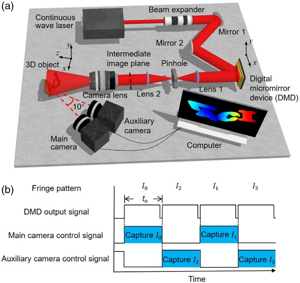
Fig. 1. Operating principle of TIA–BLIP. (a) System schematic. (b) Timing diagram and acquisition sequence. te, camera’s exposure time.

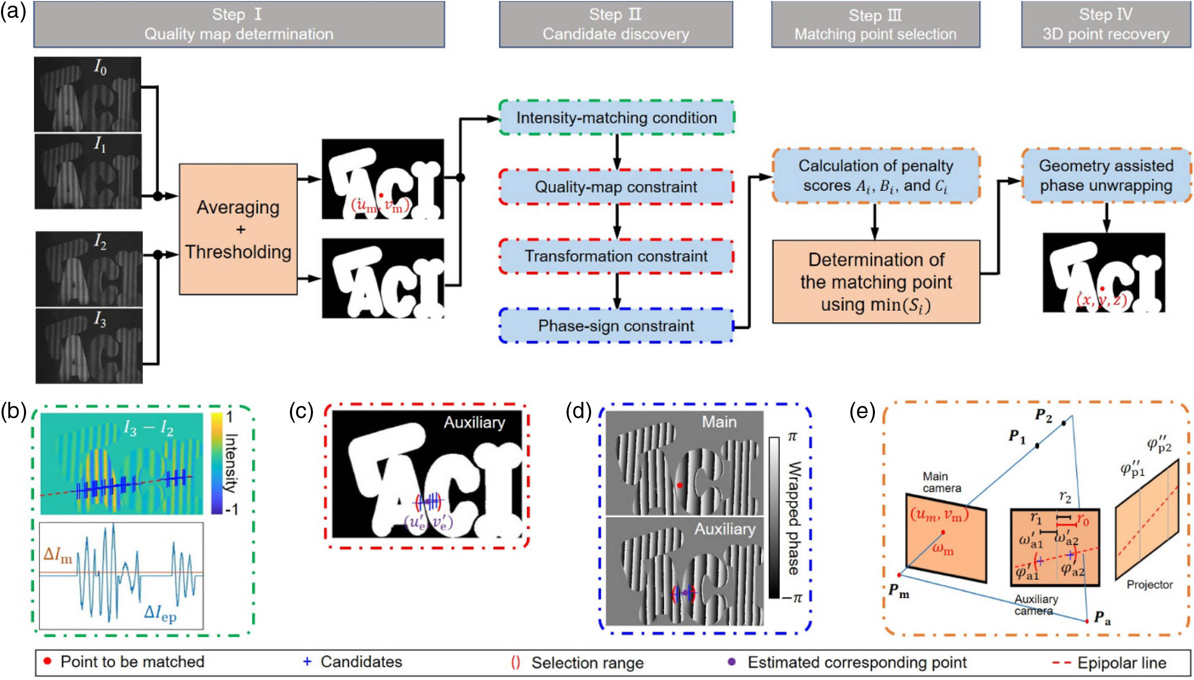
Fig. 2. Coordinate-based 3D point determination algorithm. (a) Flowchart of the algorithm. (um,vm), coordinates of the point to be matched for the main camera; (x,y,z), recovered 3D coordinates. (b) Illustrative data of the intensity matching condition. ΔIm=I0(um,vm)−I1(um,vm); ΔIep, intensity profile of I3−I2 along the epipolar line. (c) Illustrative data of the quality map constraint and the transformation constraint. (ue′,ve′), coordinates of the estimated corresponding point for the auxiliary camera. (d) Illustrative data of the phase sign constraint. (e) Scheme for penalty score calculation and phase unwrapping. ri, horizontal distance between the candidates and the estimated corresponding point; ωm, phase value of the selected point in the main camera calculated by the Fourier transform profilometry method; ωai′, phase value of the candidate points in the auxiliary camera calculated by the Fourier transform profilometry method; φai′, phase value calculated by the phase-shifting method; φpi′′, phase value determined on the projector’s plane; Pi, 3D points determined by candidates; Pm, principal point of the main camera; and Pa, principal point of the auxiliary camera.

Fig. 3. Quantification of TIA–BLIP’s depth resolution. (a) 3D images of the planar surfaces (top image) and measured depth difference (bottom plot) at four exposure times. The white boxes represent the selected regions for analysis. (b) Relation between measured depth differences and their corresponding exposure times.

Fig. 4. TIA–BLIP of static 3D objects. (a) Reconstructed results of letter toys. Two perspective views are shown in the top row. Selected depth profiles (marked by the white dashed lines in the top images) and close-up views are shown in the bottom row. (b) Two perspective views of the reconstruction results of three toy cubes.

Fig. 5. TIA–BLIP of dynamic objects. (a) Reconstructed 3D images of a moving hand at five time points. (b) Movement traces of four fingertips [marked in the first panel in (a)]. (c) Front view of the reconstructed 3D image of the bouncing balls at five different time points. (d) Evolution of 3D positions of the three balls [marked in the third panel in (c)].

Fig. 6. TIA–BLIP of sound-induced vibration on glass. (a) Schematic of the experimental setup. The field of view is marked by the red dashed box. (b) Four reconstructed 3D images of the cup driven by a 500-Hz sound signal. (c) Evolution of the depth change of five points marked in the first panel of (b) with the fitted result. (d) Evolution of the averaged depth change with the fitted results under the driving frequencies of 490 Hz, 500 Hz, and 510 Hz. Error bar: standard deviation of Δz calculated from the five selected pixels. (e) Response of the depth displacements to sound frequencies. The cyan curve is a fitted result of a Lorentz function.

Fig. 7. TIA–BLIP of glass breakage. (a) Six reconstructed 3D images showing a glass cup broken by a hammer. (b) Evolution of 3D velocities of four selected fragments marked in the fourth and fifth panels in (a). (c) Evolution of the corresponding 3D accelerations of the four selected fragments.