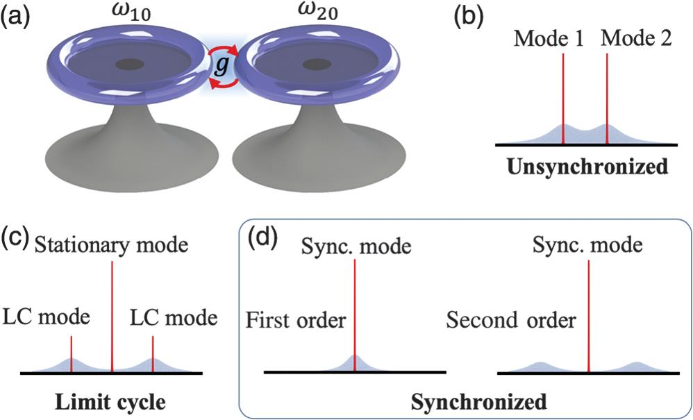
Fig. 1. Schematic diagram of the system. (a) Two detuned and self-sustained optical microcavities with different resonant frequencies, ${\omega }_{10}$ and ${\omega }_{20}$, which are directly coupled at strength $g$. (b)–(d) Frequency spectra of the coupled cavities, showing three different long-term states: unsynchronized, limit cycle (LC), and synchronized (Sync.). Light blue represents the noise backgrounds from which the first- and second-order synchronizations are distinguished.

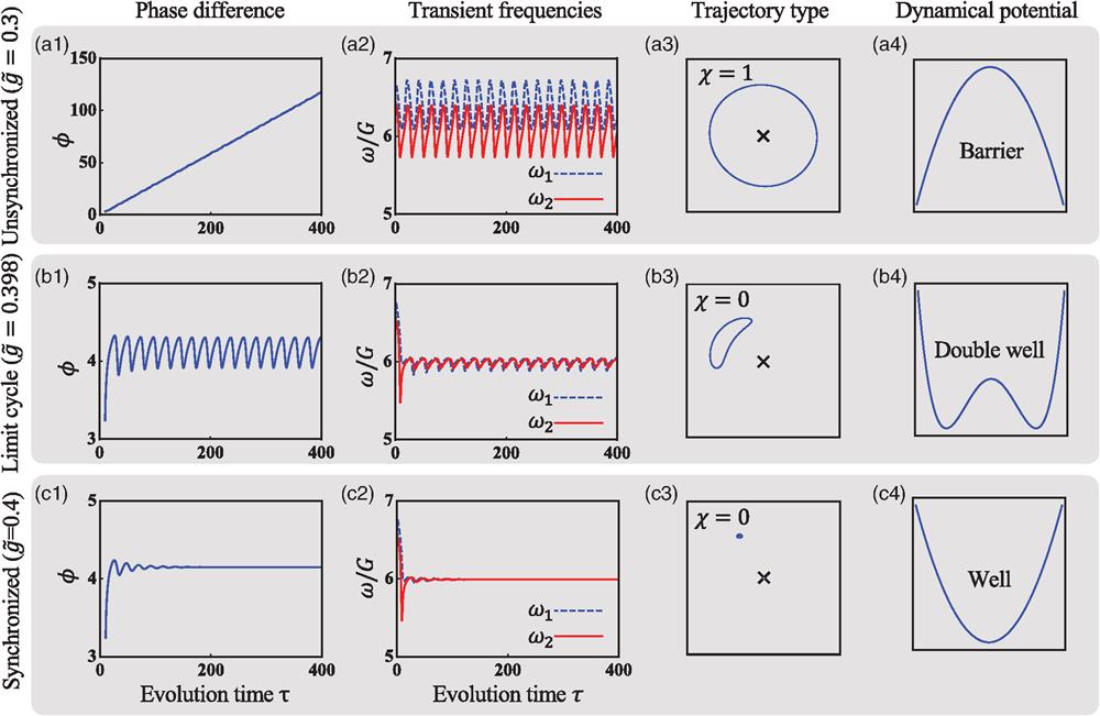
Fig. 2. Long-term evolutions of the two cavity modes under different coupling strengths. Three different categories are shown: (a) the unsynchronized ($\tilde{g}=0.3$), (b) limit cycle ($\tilde{g}=0.398$), and (c) synchronized states ($\tilde{g}=0.4$). (a1)–(c1) Phase difference; (a2)–(c2) transient frequencies; (a3)–(c3) trajectory encircling types (black cross as the axis); and (a4)–(c4) dynamical potential near the synchrony point. In all figures, the given detuning $\tilde{\mathrm{\Delta }}=0.3$ and Kerr factor $\tilde{\mathit{\delta }}=0.1$.

Fig. 3. Parameter dependence of the synchronization. (a), (b) Maximum of the frequency differences, $\max |{\omega }_1-{\omega }_2|$, versus the coupling strength $\tilde{g}$, with ($\tilde{\mathrm{\Delta }}=0.2$, $\tilde{\mathit{\delta }}=0.1$) in (a) and ($\tilde{\mathrm{\Delta }}=0.3$, $\tilde{\mathit{\delta }}=0.1$) in (b); inset shows the derivative. (c) Phase diagram in the $(\tilde{\mathrm{\Delta }},\tilde{g})$ plane with the Kerr factor $\tilde{\mathit{\delta }}=0.1$. The inaccessible (gray), limit cycle (dark blue), and synchronized (light blue) regimes are marked. The red cross stands for the triple phase point $({\tilde{\mathrm{\Delta }}}_{\mathrm{T}},{\tilde{g}}_{\mathrm{T}})$. (d) The triple phase point $({\tilde{\mathrm{\Delta }}}_{\mathrm{T}},{\tilde{g}}_{\mathrm{T}})$ depending on the Kerr factor $\tilde{\mathit{\delta }}$.

Fig. 4. Hysteresis behavior in frequency difference. (a), (b) Frequency differences $|{\omega }_1-{\omega }_2|$ versus the evolution time $\tau$ in the first- and second-order transition regimes. Insets: the real-time evolution of the coupling strength $\tilde{g}(\tau )$. (c), (d) Maxima of the frequency differences, $\max |{\omega }_1-{\omega }_2|$ versus $\tilde{g}(\tau )$. For each plot, the Kerr factor $\tilde{\delta }=0.1$; the detuning $\tilde{\mathrm{\Delta }}=0.2$ in (a) and (c), and $\tilde{\mathrm{\Delta }}=0.3$ in (b) and (d).