Synchronization is of importance in both fundamental and applied physics, but its demonstration at the micro/nanoscale is mainly limited to low-frequency oscillations such as mechanical resonators. We report the synchronization of two coupled optical microresonators, in which the high-frequency resonances in the optical domain are aligned with reduced noise. It is found that two types of synchronization regimes emerge with either the first- or second-order transition, both presenting a process of spontaneous symmetry breaking. In the second-order regime, the synchronization happens with an invariant topological character number and a larger detuning than that of the first-order case. Furthermore, an unconventional hysteresis behavior is revealed for a time-dependent coupling strength, breaking the static limitation and the temporal reciprocity. The synchronization of optical microresonators offers great potential in reconfigurable simulations of many-body physics and scalable photonic devices on a chip.
Synchronization phenomena are ubiquitously observed in nature, such as collective neuron bursts, stabilized heartbeats, and disciplined synchronous fireflies.1–3 Starting from the Huygens pendulum locked in antiphase,4,5 the synchronization of nonlinear oscillators has earned in-depth investigation.6 In daily life and modern industry, synchronization has been the basis for clock calibration, signal processing, and microwave communication,7 and provides schemes for clustered computing and memory storage.8–10 Over the past few years, the synchronization of mechanical resonators has been implemented, where the mechanical resonators are coupled strongly through direct conjunction elements,11,12 optical radiation fields,13–17 or optical traveling waves,18–21 facilitating mechanical-based high performance networks. Strong mutual coupling together with the nonlinearity of individually sustainable systems plays a crucial role in the realization of synchronization.22–27
Likewise, synchronized optical fields also promise great potential in fundamental and applied physics, such as many-body optical physics and scalable on-chip photonic devices,28–33 while the occurrence is challenged by their relatively low mutual coupling compared to the high carrier frequencies of light. Recently, microcomb solitons have been experimentally synchronized,34,35 significantly expanding their photonic applications, yet the repetition rates in the range of microwaves rather than the optical frequency of the comb lines are equalized. In this article, we discuss the mode synchronization of two optical microresonators without an external reference frequency, where the distant modes are self-sustained and mutually aligned through a weak coupling. The synchronization results from the spontaneous symmetry breaking and takes the form of a first- or second-order transition. Furthermore, an unconventional hysteresis behavior is presented as the coupling strength varies, permitting nonreciprocal synchronization in a more extensive parametric space.
2 Results
2.1 Two Self-Sustained Microresonators and Interaction Model
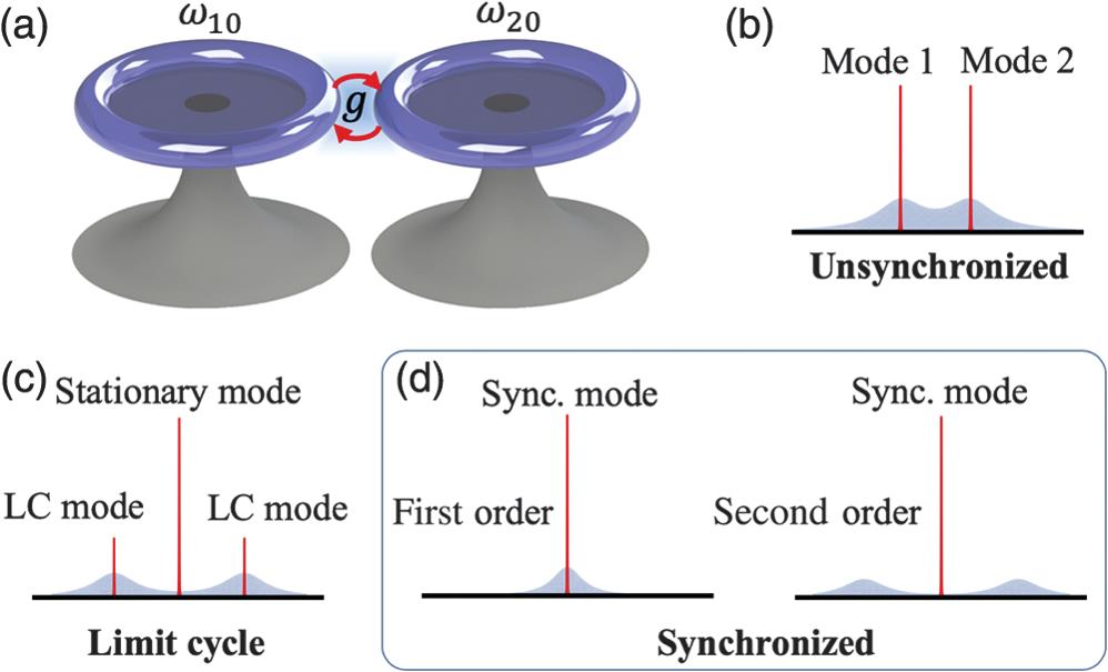
As shown in Fig. 1(a), the system is composed of two optical microcavities with different resonant frequencies, and , coupled at the strength . The ’th () cavity is self-sustained by the internal gain described by the factor and the intrinsic dissipation at the rate . In the presence of nonlinear gain, a self-Kerr type modulation is present, with being the annihilation operator and the factor describing the self-Kerr effect.36 With the gain saturation37 or the multiphoton absorption,38–40 the effective dissipation of the ’th mode is modeled as , where is the nonlinearity factor.
Sign up for Advanced Photonics TOC. Get the latest issue of Advanced Photonics delivered right to you!Sign up now
Figure 1.Schematic diagram of the system. (a) Two detuned and self-sustained optical microcavities with different resonant frequencies, and , which are directly coupled at strength . (b)–(d) Frequency spectra of the coupled cavities, showing three different long-term states: unsynchronized, limit cycle (LC), and synchronized (Sync.). Light blue represents the noise backgrounds from which the first- and second-order synchronizations are distinguished.
The dissipative evolution of the system is described by the Lindblad density-matrix equation ( hereafter), Here, and denote the net gain factor. Without an external frequency reference, the time-independent Hamiltonian ⏧⏧⏧⏧, under the rotating-wave approximation. For simplicity, in the following we set , , and ; the dimensionless parameters are defined as , , and . The time scale . These formalisms can be checked from wave functions in systems such as coupled laser systems.41,42 Though the coupling between the two modes is linear and energy-conservative, it plays the role of messenger passing over the weak and detuned drive. The self-sustained system always favors the resonance mutual driving, and the synchronization of the two modes is established by the spontaneous frequency alignment of the individual cavities, through the self-Kerr effect and the amplitude stabilization under the saturation effect. In this way, the modes are synchronized in individual cavities.
2.2 Synchrony Solution in Static Case
We focus on the phase difference and the transient frequencies of two modes in the coherent-state representation.6 In this representation, the complex amplitude is parameterized as , where and are the amplitude and the phase, respectively. Let be the phase difference, which is the preserved degree of freedom, and let be the transient frequency for the ’th mode.
Following the standard Wigner function formalism,43 the mode equation is described by , where and denote the quasiprobability drift flow of the two modes (see Supplementary Material for details). The synchrony solution is achieved when , and a fixed point emerges in the parametric space (see Supplementary Material for details). In Fig. 2, we plot the phase differences and the transient frequencies for different . Three categories of long-term behaviors are discovered. When the coupling strength is low, , for example, the phase difference accumulates to infinity quickly [see Fig. 2(a1)], and the transient frequencies and are effectively separated [Fig. 2(a2)], showing two separated modes in the frequency spectrum [Fig. 1(b)]. When the coupling strength is turned higher, , for example, the phase difference vibrates around the stationary point but does not accumulate [Fig. 2(b1)], and the frequencies and breathe slowly around the stationary frequency [Fig. 2(b2)], generating a limit cycle state. A stationary mode is localized around the original two cavity modes, and a pair of weak limit cycle modes can be found symmetrically detuned from the stationary modes [Fig. 1(c)]. Finally, with a high enough coupling strength, such as , the phase difference stabilizes [Fig. 2(c1)], and the frequencies and also converge to a single value [Fig. 2(c2)], reaching the synchronized state with a single mode in the frequency spectrum [Fig. 1(d)].
Figure 2.Long-term evolutions of the two cavity modes under different coupling strengths. Three different categories are shown: (a) the unsynchronized (), (b) limit cycle (), and (c) synchronized states (). (a1)–(c1) Phase difference; (a2)–(c2) transient frequencies; (a3)–(c3) trajectory encircling types (black cross as the axis); and (a4)–(c4) dynamical potential near the synchrony point. In all figures, the given detuning and Kerr factor .
It is noted that the temporal translational symmetry (TTS) is preserved in the synchronized state because both the amplitudes and phase difference remain invariant while the symmetry is broken in the unsynchronized and limit cycle states. The discrete topological character number as the average encircling number is further defined as with being the period of long-term evolution (see Supplementary Material for details).44 As shown in Fig. 2(a3), the unsynchronized trajectory encircles the axis and has the character number . The later two categories of trajectories, the off-axial circles [Fig. 2(b3)] and the fixed points [Fig. 2(c3)], have the character number (see the transformed space in Supplementary Material for details). With the different symmetries and character numbers, the three long-term states are classified accordingly (see Supplementary Material for details).
2.3 Analysis of Different Transition Types
When we further study the maximum of the frequency differences, , two types of synchronization transitions are found. As shown in Fig. 3(a), when the coupling strength is low, the maximal frequency difference varies slowly. At a critical strength , it suddenly falls to zero, which shows the characteristics of the first-order transition. As shown in Fig. 3(b), the maximal frequency difference continuously decreases to zero but has a discontinuity in its derivative at , showing the feature of the second-order transition. In addition, the noise spectrum is also calculated in long-term motions. For the synchronized spectrum in Fig. 1(d), the background noise has coinciding peaks with synchronized frequencies in the first-order transition, whereas the noise has shifted-away peaks in the second-order transition (see Supplementary Material for details).
Figure 3.Parameter dependence of the synchronization. (a), (b) Maximum of the frequency differences, , versus the coupling strength , with (, ) in (a) and (, ) in (b); inset shows the derivative. (c) Phase diagram in the plane with the Kerr factor . The inaccessible (gray), limit cycle (dark blue), and synchronized (light blue) regimes are marked. The red cross stands for the triple phase point . (d) The triple phase point depending on the Kerr factor .
In order to study the critical coupling strength and the transition behaviors in its vicinity, a real-valued dynamical potential is defined (see Supplementary Material for details). Only if the dynamical potential has a local minimum, the fixed point emerges and remains stable, and thus indicates the existence of a synchronized state (see Supplementary Material for details). In the vicinity of the fixed point, the dynamical potential can be expanded as , where is the Jacobian matrix, is the arbitrarily small displacement from the fixed point, and H.c. is the Hermitian conjugate. The displacement signifies the breaking of the TTS. At , the TTS is preserved. The stability near the fixed point is thus governed by the eigenvalues of the Jacobian. When the largest real part of the eigenvalues [known as the largest Lyapunov exponent ] is positive, the fixed point is unstable and vice versa (see Supplementary Material for details).45 The critical coupling strength is then taken at .
In the three-dimensional space , the Jacobian has purely real components, and thus the complex eigenvalues must come in pairs. If the largest Lyapunov exponent equals one of the eigenvalues, the dynamical potential is simplified as where is the perturbation of in the direction of corresponding eigenvector, and the real coefficient (see Supplementary Material for details). It is noted that the dynamical potential in Eq. (3) becomes a well or a barrier depending on or , which leads to the synchronized or unsynchronized state shown in Figs. 2(a4) and 2(c4). Thus, the first-order transition happens at , explaining the sudden convergence of frequency difference in Fig. 3(a). For and , the TTS is broken () and preserved (), respectively. If the largest Lyapunov exponent equals the real parts of a pair of conjugating eigenvalues, the averaged dynamical potential is where is the radial displacement from and the real coefficients (see Supplementary Material for details).46 When , a double-well type potential is obtained, corresponding to the limit cycle state shown in Fig. 2(b4). After surpasses , the averaged dynamical potential has a single local minimum at , and the synchronization is reached, accounting for the second-order transition depicted in Fig. 3(b). The TTS is spontaneously broken as the radial displacement continuously departs from the synchrony point .
In the light of the static analysis above, the phase diagram in the -cross section is plotted in Fig. 3(c), where three regions of different long-term behaviors are marked. The synchronized and limit cycle regimes are specified according to the existence of a single and double local minima of the dynamical potentials, respectively. The inaccessible (unsynchronized) regime corresponds to the saddle nodes in the dynamical potentials, and thus neither the synchronized state nor the limit cycle state can survive in this regime. The transition from the unsynchronized state to the synchronized state is of first-order and has a variant topological character number. The transition from the limit cycle state to the synchronized state is of second-order and has an invariant topological character number (see Supplementary Material for details). It is also found that a triple phase point emerges at and , where is the minimal detuning required for the second-order transition. This point corresponds to the solution where two eigenvalues of the Jacobi matrix are zeros. For the detuning (), the first-order (second-order) transition happens around (black solid line). The triple phase point relies crucially on the strength of the Kerr effect. In Fig. 3(d), we plot and with respect to the Kerr factor , showing monotone increasing and decreasing dependence, respectively. When the factor increases, the self-tuning ability of the Kerr effect is strengthened, and the second-order synchronization under a larger detuning and a weaker coupling becomes possible.
2.4 Hysteresis Behavior
The two types of synchronization transitions present distinct hysteresis behaviors near the critical coupling strength . In Fig. 4, the frequency differences and their maxima, , are plotted, to indicate when the real-time coupling strength slowly increases (forward) and then decreases (backward). In the first-order transition regime, whatever direction moves, the synchronization emerges or disappears at the same as derived in the static analysis [see Fig. 4(a)]. The maximal frequency differences in the forward and backward evolutions are identical to those depicted in Fig. 4(c), coinciding with Fig. 3(a). In the second-order transition regime, although the synchronization also emerges at in the forward trip, it does not disappear at the same critical point in the backward trip [see Fig. 4(b)]. Actually, the synchronization survives far below , even into the statically inaccessible region depicted in Fig. 3(c). Further calculation of the maximal frequency differences reveals a hysteresis loop in this case [see Fig. 4(d)]. The forward half of the loop remains the same as the curve in Fig. 3(b), whereas the backward half is beneath it. The critical coupling strength under the static model does not apply under a dynamical model with the second-order transition. As explained in the Supplementary Material,47 the passes with the emergence of new non-zero eigenvalues proportional to . This mechanism is thus attributed to the singularity of and the altering direction of real-time . The hysteresis property breaks the minimal coupling required for the synchronization, and the consequent temporal nonreciprocity enables the reading out of coupling history as has been done in the ferromagnetic materials.48
Figure 4.Hysteresis behavior in frequency difference. (a), (b) Frequency differences versus the evolution time in the first- and second-order transition regimes. Insets: the real-time evolution of the coupling strength . (c), (d) Maxima of the frequency differences, versus . For each plot, the Kerr factor ; the detuning in (a) and (c), and in (b) and (d).
In summary, we have presented the mode synchronization of two self-sustained optical microresonators that are largely detuned and linearly coupled together. The synchronization is accompanied by a process of spontaneous symmetry breaking, taking the form of the first- and second-order transitions. First, when the synchronization takes place, the high transient frequencies of both modes collapse, offering a possible solution to the frequency mismatch problem in integrating optical microresonators. The phase noise of the coupled system is dramatically reduced, revealing spontaneous symmetry preservation and paving the way for error-tolerant device fabrication.19 Second, the topological character transitions cast light on many-body physics. The experimental realization can be approached by coupling two toroid cavities etched with the same mask. Raman gain is applied separately to each cavity at tunable pump frequencies. With additional thermal control of the refractive index, perfect phase matching and adjustable mode frequency differences are achievable. Note that in our model the evolution in the transformed space corresponds to the nontrivial degeneration of a ring into a point. During the synchronization of three resonators, however, the transition also includes nontrivial degeneration of the torus into a ring. The multiple-torus topological structure in massively coupled resonators offers new insights for many-body physics.49 Finally, in the second-order transition regime, an unconventional hysteresis behavior was predicted, breaking the static critical coupling strength limit. The coupling history of the resonators can be logged over a short period autonomously, which is desirable in all-optical memory designs.50,51 These results thus show great potential for further research studies in all-optical memory, coupled cavity quantum electrodynamics, and many-body optical physics.