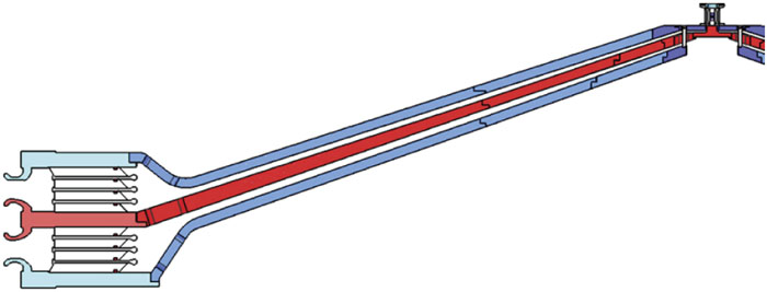
Fig. 1. (a) Schematic of the full double-disk MITL that shows the insulator stack, the vacuum flare region, the MITLs, the post-hole convolute, the inner disk MITL, and the load region. (b) Schematic showing the dimensions of the two MITLs being modeled. The 1.5-Ω impedance value is only for the radius and gap at that point. The vertical scale is expanded four times for clarity.

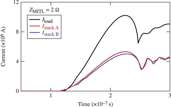
Fig. 2. Calculated total current (black solid curve), A-level current (red solid curve), and B-level current (blue solid curve) as functions of time.

Fig. 3. Calculated currents in each MITL segment as functions of time. The differences seen in the time window from 120 ns to 140 ns reflect losses during the setup of magnetic insulation.

Fig. 4. Calculated voltages in each MITL segment as functions of time.

Fig. 5. Electron-loss currents in each MITL segment, where the largest current losses occur with the inner MITL segment 10. z-pinch stagnation is at ∼255 ns.

Fig. 6. Electron-loss current density in each MITL segment, where the largest current density losses occur with the inner MITL segment 10.

Fig. 7. Calculated total current (black solid curve), A-level current (red solid curve), and B-level current (blue solid curve) as functions of time.

Fig. 8. Calculated currents in each MITL segment as functions of time for the variable-impedance MITL. The differences in the various currents seen at ∼120 ns to 150 ns reflect losses during the setup of magnetic insulation.

Fig. 9. Calculated voltages of each MITL segment with time. The voltages decrease radially inward.

Fig. 10. Electron-loss currents in each MITL segment for the variable-impedance MITL, where the largest current losses occur with inner MITL segment 10. z-pinch stagnation is at ∼255 ns.

Fig. 11. Electron-loss current density in each MITL segment of the variable-impedance MITL, where the largest current-density losses occur with inner MITL segment 10.

Table 1. Listing of the MITL parameters from the ten MITL segments on the B level from SCREAMER calculations for a 2-Ω constant-impedance MITL.

Table 2. Radius, circumference, gap, impedance, and inductance of the ten MITL segments used in the SCREAMER calculations.

Table 3. Listing of B-level MITL parameters from SCREAMER calculations for a variable-impedance MITL.