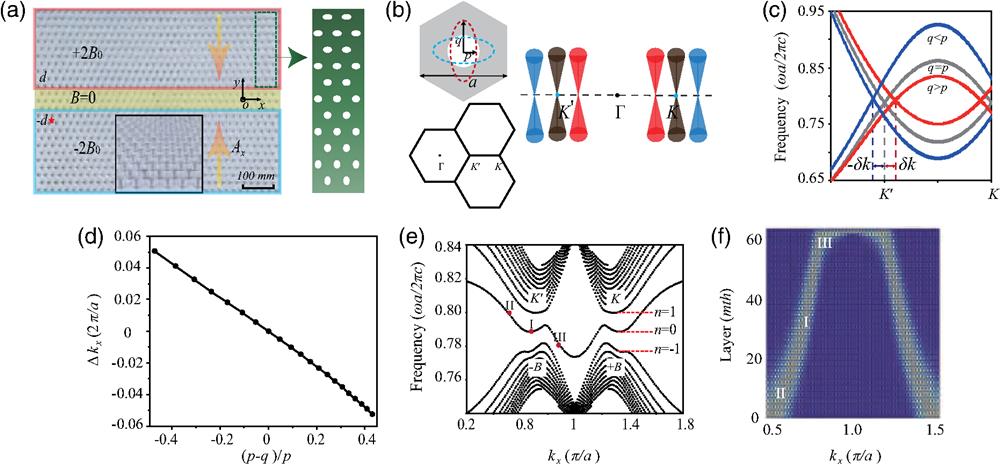
Fig. 1. (a) Experimental sample of a heterostructure with nonuniform PMFs, consisting of two reversed gradient PhCs and a transition region. The PMF applied perpendicular to the PhCs is zero in the central yellow region, while has the opposite direction with the same magnitude in the upper and lower half parts. The sign of the PMF is referred to the K valley. (b) Left panel: Schematic of the unit cell of the PhC and the Brillouin zone with high symmetry points Γ, K, and K′. Right panel: shift of Dirac cones at K and K′ valleys when metallic cylinders are deformed into elliptical shapes. (c) Band structure of the PhC with different sizes of metallic pillars. (d) Linear relation between (p−q)/p and the shift of Dirac points represented by δkx. (e) LLs of a gradient PhC under a strong PMF. (f) Distribution of eigen-electric fields of n=0 LL and the edge states as a function of wave vector kx.

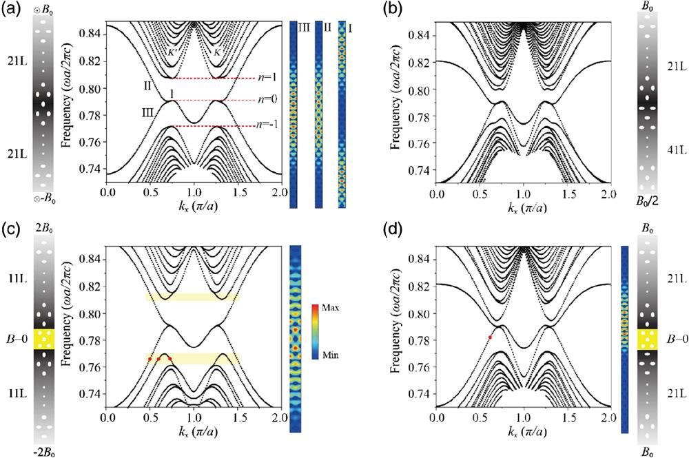
Fig. 2. (a) Quantization of LLs of two reversed gradient PhCs with M=21 layers possessing antiparallel PMFs for σ=−1. Right panel: distributions of eigen-electric fields. I: n=0 LL at k=0.75(π/a) and normalized frequency f=0.791c/a. II and III: edge states at k=0.6(π/a) and f=0.783, 0.796c/a. (b) LLs in a heterostructure with the same sign but unequal PMFs. The upper and lower regions have 21 and 41 layers, respectively, for σ=0.5. (c) Snake state in a nonuniform PMFs with M=11 layers at each gradient PhC. Right panel: electric field distribution of snake state at k=0.6(π/a) and f=0.766c/a. (d) Dispersive LLs in a heterostructure with parallel PMFs at two PhCs without the snake state dispersion for σ=1. Right panel: electric field distribution at k=0.6(π/a) and f=0.780c/a.

Fig. 3. (a) Experimental sample of two reversed gradient PhCs. Red and blue stars indicate the positions of the excited source. (b) and (c) Simulated distributions of electric fields of edge states at the top and bottom boundaries of a gradient PhC, corresponding to 10.72 and 11.0 GHz, respectively. (d) Experimental measurement of the edge state at the top boundary at 10.7 GHz. (e) Defined parameter Cs denotes the confinement of the edge state. (f) and (g) Transmission spectra in the simulation and experiment.

Fig. 4. (a) and (b) Distributions of the electric field of the large-area interface state in the simulation and experiment at 11.12 and 11.30 GHz, respectively. The measured region of the electric field is a part of the simulated region and PhC sample. (c) and (d) Normalized electric field intensity along the y direction at x=490 and 560 mm.

Fig. 5. (a) and (b) Electric field distributions of the snake state at 10.42 and 10.30 GHz in the simulation and experiment, respectively. (c) Propagation of the snake state under the disorder realized by moving the position of metallic pillars. (d) and (e) Simulated and experimental electric field intensities along the y direction.