Statistical and quantum photoionization cross sections in plasmas: Analytical approaches for any configurations including inner shells

F. B. Rosmej; L. A. Vainshtein; V. A. Astapenko; V. S. Lisitsa

doi:10.1063/5.0022751

Abstract

Statistical models combined with the local plasma frequency approach applied to the atomic electron density are employed to study the photoionization cross-section for complex atoms. It is demonstrated that the Thomas–Fermi atom provides surprisingly good overall agreement even for complex outer-shell configurations, where quantum mechanical approaches that include electron correlations are exceedingly difficult. Quantum mechanical photoionization calculations are studied with respect to energy and nl quantum number for hydrogen-like and non-hydrogen-like atoms and ions. A generalized scaled photoionization model (GSPM) based on the simultaneous introduction of effective charges for non-H-like energies and scaling charges for the reduced energy scale allows the development of analytical formulas for all states nl. Explicit expressions for nl = 1s, 2s, 2p, 3s, 3p, 3d, 4s, 4p, 4d, 4f, and 5s are obtained. Application to H-like and non-H-like atoms and ions and to neutral atoms demonstrates the universality of the scaled analytical approach including inner-shell photoionization. Likewise, GSPM describes the near-threshold behavior and high-energy asymptotes well. Finally, we discuss the various models and the correspondence principle along with experimental data and with respect to a good compromise between generality and precision. The results are also relevant to large-scale integrated light–matter interaction simulations, e.g., X-ray free-electron laser interactions with matter or photoionization driven by a broadband radiation field such as Planckian radiation.

I. INTRODUCTION

Most of the matter in the universe is ionized and in the so-called plasma state.^1–3 There are essentially two main sources of ionization: collisional ionization due to particle impact (by electrons, atoms, and ions) and photoionization. In astrophysical plasmas, including astrophysical laboratory plasmas, photoionization of radiation fields drives important plasma ionization.^4–7 The photoionization rate and the ionization degree of the plasma depend on the nature of the radiation sources, in particular on the spectral distribution of the photon intensity and the photoionization cross-sections.

In inertial confinement fusion, megajoule laser irradiation of the inner walls of the hohlraum creates a radiation field that in turn results in the implosion of the deuterium–tritium (DT) capsule.^7,8 To create the most homogenous implosion conditions, a near-Planckian radiation field is envisaged.

For laboratory studies, the rapid development of laser-driven light sources, i.e., higher-harmonic generation (HHG),⁹ as well as extreme ultraviolet (XUV)/X-ray free-electron lasers (XUV-FEL/XFEL),^10–12 has stimulated particular interest in the photoionization of inner atomic and ionic shells. In fact, owing to the high laser intensity at X-ray energies, photoionization of inner atomic shells by XFEL radiation is the primary source of matter heating: for example, in XFEL–solid matter interaction when microfocusing is applied, the photon density in the light pencil is near solid density. As almost all inner shells in the lattice are photoionized (a so-called hollow crystal), massive numbers of photoelectrons are generated, which are followed by Auger electrons. Owing to the large number of Auger electrons, significant heating is initiated; this is so-called Auger electron heating.^13–16 Moreover, owing to the high electron density in the conduction band, the heating is amplified by three-body recombination heating.¹⁷ Therefore, simulation of XFEL interaction with solids requires expressions for photoionization cross-sections from all configurations, including in particular inner atomic shells.^15,18

Similar considerations hold true for high-energy-density physics, where intense radiation fields drive important matter ionization: general expressions for the photoionization cross-sections from any configurations of rather complex atoms and ions are required in order to realize large-scale integrated simulations in light–matter interaction physics.

It is therefore the aim of the present work to develop various methods that are suitable for general implementation in integrated simulations in which a reasonable compromise between generality and precision can be achieved. In Sec. II, we present an introduction to the photoionization processes in a quantum mechanical approach, including the continuum oscillator strengths, the Born relation, the plasma frequency approach, and the mixed quantum–classical approach. In Sec. III, we present studies of photoionization for H-like atoms and discuss important scaling relations. We present quantum mechanical numerical calculations in Sec. IV, where we also propose generalized scaled analytical photoionization cross-section formulas for any configuration. In Sec. V, we consider inner-shell photoionization. We present a comparison with experimental data in Sec. VI, where we also discuss various types of models in the plasma frequency approach. In Sec. VII, we summarize formulas for the photoionization rates for different types of radiation fields. This is followed by the conclusion in Sec. VIII.

II. GENERAL RELATIONS AND APPROXIMATIONS

A. Quantum mechanical approach and continuum oscillator strength

Let an atom be excited as a result of absorption of a photon of an external field. Photoabsorption is characterized by a spectral cross-section that is connected with the probability per unit time for excitation of a bound electron under the action of electromagnetic radiation with a specified frequency ω. It is convenient to express the value σ(ω) in terms of the spectral function of dipole excitationsg(ω):¹⁹ $\begin{matrix} σ (ω) = \frac{2 π^{2} a_{0}}{c} g (ω), \end{matrix}$ (2.1)where a₀ = 0.529 × 10⁻⁸ cm is the Bohr radius and c is the speed of light (note that the speed of light in atomic units is c/V₀ = 1/α ≈ 137, where V₀ ≅ 2.18 · 10⁸ cm/s is the velocity of an electron in the first Bohr orbit in a hydrogen atom, i.e., an atomic unit of velocity, and α = e²/ℏc = 1/137.036 is the fine structure constant). The function g(ω) is very convenient, because it satisfies the sum rule $\begin{matrix} \int g (ω) d ω = N_{n}, \end{matrix}$ (2.2)where N_n is the total number of electrons in an atom in shell n. Besides, the spectral function g(ω) also satisfies the equation $\begin{matrix} g (ω) = \sum_{j} f_{i j} δ (ω - ω_{i j}), \end{matrix}$ (2.3)where f_ij is the strength of an oscillator for the transition i → j and ω_ij is the eigenfrequency of this transition. Equations (2.1)–(2.3) apply not only to photoabsorption but also to photoionization. In the case of photoionization, the summation in Eq. (2.3) is replaced by an integration over states of the continuous spectrum, the integrand being a differential oscillator strength for transition to the continuum, df/dε, where ε is the energy of a state of the continuous spectrum of an electron. The differential oscillator strength is expressed in terms of the matrix element d_iε of a transition dipole moment operator for transitions to the continuum in the same manner as for transitions to the discrete spectrum: $\begin{matrix} \frac{d f}{d ε} = \frac{2 ω {∣d_{i ε}∣}^{2}}{3 e^{2} a_{0}^{2}}, \end{matrix}$ (2.4)where e is the elementary charge. The oscillator strength of such transitions has to be divided by the energy interval from the given level to the nearest energy level. It can be shown that in this case the following relation is valid:^20–22 $\begin{matrix} \underset{n^{'} \to \infty}{l i m} \frac{2 π^{2}}{c} a_{0}^{2} 2 R y \frac{f_{n l, n^{'} l^{'}}}{E_{n^{'} + 1 l^{'}} - E_{n^{'} l^{'}}} = σ_{n l, ε l^{'}} (I_{n l}) . \end{matrix}$ (2.5)This means that the normalized oscillator strength density for infinitely large principal quantum numbers goes over to the threshold value of the partial (corresponding to a given value of orbital quantum number l′) cross-section of photoionization of an electron subshell nl. The limiting transition (2.5) demonstrates a smooth conjugation of optical characteristics of discrete and continuous spectra.

The most general expression for the cross-section for photoionization of an electron subshell in the one-electron approximation (i.e., with interelectron correlations neglected) has the form $\begin{matrix} σ_{n l} (ω) = \frac{4 π^{2} N_{n l}}{3 e^{2} a_{0} ω c (2 l + 1)} [{∣d_{n l, ε (l + 1)}∣}^{2} + {∣d_{n l, ε (l - 1)}∣}^{2}], \end{matrix}$ (2.6)where N_nl is the number of equivalent electrons, i.e., electrons with the same values of principal and orbital quantum numbers. This expression involves the matrix elements of a dipole moment operator for transitions to states of the continuous spectrum with orbital quantum numbers allowed by selection rules. These matrix elements can be expressed in terms of radial wave functions of the initial, R_nl(r), and final, $R_{e l^{'}} (r),$ states as follows: $\begin{matrix} d_{n l, ε l^{'}} & = \frac{e V_{0}}{a_{0}} \sqrt{(2 l + 1) (2 l^{'} + 1)} (\begin{matrix} \begin{matrix} l & 1 & l^{'} \end{matrix} \\ \begin{matrix} 0 & 0 & 0 \end{matrix} \end{matrix}) \\ \times \int_{0}^{\infty} R_{n l} (r) r R_{ε l^{'}} (r) r^{2} d r, \end{matrix}$ (2.7)where $(\begin{matrix} \begin{matrix} l & 1 & l^{'} \end{matrix} \\ \begin{matrix} 0 & 0 & 0 \end{matrix} \end{matrix})$ is the so-called 3j symbol, which results from integration with respect to angular variables in the definition of the matrix element of the dipole moment. The 3j symbol describes the selection rules for dipole radiation, according to which l′ = l ± 1. Naturally, in the case l = 0, there is one allowed value of a quantum number of an orbital moment in the final state: l′ = 1. As a rule, the main contribution to the photoionization cross-section is made by a transition with increasing quantum number of an orbital moment, l → l + 1. Exceptions to this rule occur if for some specific reasons the matrix element $d_{n l, n^{'} l + 1}$ is small or goes to zero. On the other hand, for the angular distribution of ionized electrons (which we do not consider here), the transition l → l − 1 can play an important role.

B. Born approximation

For small values of the Born parameter ζ = z/ka₀ = ze²/ℏV ≪ 1 (where z is the charge of the ion, the spectroscopic symbol), the influence of the atomic core on the motion of an ionized electron can be considered to be a small perturbation. This is the case for high velocities and low nuclear charges. In this case, plane waves corresponding to free motion can be used as the wave functions of ionized electrons in the calculation of the matrix elements d_nl,εl+1 appearing in the general formula (2.6) for the photoionization cross-section. Then, the following expression can be obtained for the photoionization cross-section of an atomic subshell: $\begin{matrix} σ_{n l} (ω) = \frac{8 π^{2}}{3 c} N_{n l} a_{0}^{2} \frac{R y}{ℏ ω} {(\frac{p (ω)}{ℏ})}^{3} | {g_{n l} (\frac{p (ω)}{ℏ}) |}^{2}, \end{matrix}$ (2.8)where $p (ω) = \sqrt{2 m (ℏ ω - I_{n l})}$ is the momentum of the ionized electron, I_nl is the ionization potential of the electron subshell, $\begin{matrix} g_{n l} (k) = \sqrt{\frac{2}{π}} \int_{0}^{\infty} j_{l} (k r) R_{n l} (r) r^{2} d r \end{matrix}$ is the Fourier transform of the radial wave function of the initial state of the atom, R_nl(r) is the radial wave function of the initial state of an atomic electron normalized according to $\int_{0}^{\infty} {∣R_{n l} (r)∣}^{2} r^{2} d r = 1$ , and j_l(kr) is the spherical Bessel function of order l.

To clarify the notation, we give for reference several spherical Bessel functions: j₀(x) = sin x/x, j₁(x) = sin x/x² − cos x/x, j₂(x)=(3x⁻³ − x⁻¹)sin x − 3cos x/x². Spherical Bessel functions describe the radial dependence of a spherical wave with a specified value of the orbital quantum number l.

In the case of ground-state photoionization of a hydrogen atom, we have $\begin{matrix} R_{10} (r) & = (2 / \sqrt{a_{0}^{3}}) \exp (- r / a_{B}), g_{10} (k) \\ = \sqrt{\frac{2}{π}} \frac{4 a_{0}^{3 / 2}}{{(1 + k^{2} a_{0}^{2})}^{2}}, N_{n l} = 1, I_{n l} = R y . \end{matrix}$

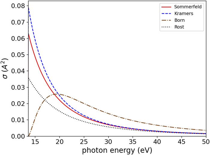
Substituting these expressions into Eq. (2.8), we find the following expression for the photoionization cross-section of a hydrogen atom in the Born approximation: $\begin{matrix} σ_{1 s}^{(B)} (ω) = \frac{2^{8} π}{3 c} a_{0}^{2} \frac{R y}{ℏ ω} \frac{{(p (ω) a_{0} / ℏ)}^{3}}{{[1 + {(p (ω) a_{0} / ℏ)}^{2}]}^{4}} . \end{matrix}$ (2.9)

A plot of the function $σ_{1 s}^{(B)} (ω)$ is presented in Fig. 1 as the dash-dotted curve.

Figure 1.The Sommerfeld, Kramers, and Born cross-sections for photoionization of the ground state of a hydrogen atom and the cross-section in the Rost approximation vs the photon energy. The cross-sections are in units of Å² = 10⁻¹⁶ cm².

A characteristic feature of the Born cross-section can be seen in Fig. 1: it goes to zero at the threshold, in contrast to the exact Sommerfeld cross-section and the approximate Kramers cross-section, both of which have their maximum values at the threshold. This is connected with the fact that the Born approximation does not take into account nuclear attraction, which increases the value of the cross-section. On the other hand, the function (2.9) has the correct high-frequency asymptotic behavior $σ_{1 s}^{(B)} (ℏ ω > > R y) \propto ω^{- 7 / 2}$ , since in the mode of high photon energies, an ionized electron can be considered to be free, which corresponds to the condition of applicability of the Born approximation. Nevertheless, the ratio of the Born cross-section to the exact cross-section at ℏω = 100 eV is 2.1, at ℏω = 1 keV, it is 1.38, and only at ℏω = 10 keV is this ratio equal to 1.12; i.e., the convergence is rather slow. It is interesting to note that for not too high photon energies, the classical Kramers photoionization cross-section (see the Sec. VI below) for a hydrogen atom describes the real situation better than the Born cross-section.

C. Local plasma frequency model

So far, the photoionization cross-section has been calculated with neglect of interelectron interaction; i.e., it has been assumed that photon absorption occurs as a result of interaction of an electromagnetic field with individual electrons, the contributions of which are additively summed, giving the total cross-section. There is a rather simple alternative approach to the description of atomic photoionization based on purely classical considerations. This is the local plasma frequency model or the Brandt–Lundqvist approximation.²³ Within the framework of this approach, an atom is approximated by an inhomogeneous distribution of electron density with concentration n(r) (plus nucleus). Each spatial point corresponds to its own local plasma frequency $ω_{p} (r) = \sqrt{4 π e^{2} n (r) / m}$ , and interaction of an external electromagnetic field of frequency ω with atomic electrons is defined by the plasma resonance condition [in atomic units, i.e., with ω in units of 2Ry and n(r) in units of $1 / a_{0}^{3}$ ] $\begin{matrix} ω = ω_{p} (r) = \sqrt{4 π n (r)} . \end{matrix}$ (2.10)It follows from this equation that absorption of electromagnetic field energy by atomic electrons occurs at those distances from a nucleus where the local plasma frequency coincides with the ionizing radiation frequency. This model results in the following simple expression for the spectral function: $\begin{matrix} g (ω) = \int d^{3} r n (r) δ (ω - ω_{p} (r)) . \end{matrix}$ (2.11)It is easy to see that the spectral function (2.11) satisfies the sum rule (2.2). For the photoionization cross-section, according to (2.1), we have $\begin{matrix} σ (ω) = \frac{2 π^{2}}{c} a_{0} \int d^{3} r n (r) δ (ω - ω_{p} (r)) . \end{matrix}$ (2.12)The presence of the delta function in Eq. (2.12) allows easy integration with respect to spatial variables. As a result, we obtain the so-called Brandt–Lundqvist approximation for the photoionization cross-section: $\begin{matrix} σ_{p h}^{B - L} (ω) = \frac{4 π^{2} ω}{c} r_{ω}^{2} \frac{n (r_{ω})}{∣n^{'} (r_{ω})∣}, \end{matrix}$ (2.13)where r_ω is the solution of Eq. (2.10). This value corresponds to the radial distance (from the nucleus) of the plasma resonance, and the prime denotes differentiation with respect to the radius. Thus, within the framework of the model, the photoionization cross-section is defined only by the distribution of the electron density n(r). For this last value, it is convenient to use the statistical model of an atom, in which $n (r) = (Z^{2} / a_{B}^{3}) f (x = r / r_{T F})$ , where f(x) is a universal function of the reduced distance x = r/r_TF, Z is the nuclear charge, and $r_{T F} = b a_{0} / Z^{1 / 3}$ is the Thomas–Fermi radius, with b ≅ 0.8853. Substituting this expression for the electron density into Eq. (2.13), we find $\begin{matrix} σ_{p h}^{B - L} (ω) = s (ν = \frac{ℏ ω}{2 Z R y}) = \frac{9 π^{4} ν}{32 c} x_{ν}^{2} \frac{f (x_{ν})}{∣f^{'} (x_{ν})∣} a_{0}^{2}, \end{matrix}$ (2.14)where the reduced frequency ν = ℏω/(2ZRy) has been introduced, and x_ν is the solution of the equation $ν = \sqrt{4 π f (x)}$ that is a consequence of Eq. (2.10).

As can be seen from Eq. (2.14), the photoionization cross-section in the Brandt–Lundqvist approximation is found to be a universal function, that is to say, it is independent of nuclear charge but a function of the reduced frequency: s(ν). Equation (2.14) reveals the corresponding scaling law for the cross-section with respect to the variable ν. The universal function s(ν) is defined by the type of statistical model of the atom, i.e., by the dependence of f(x). Figure 2 shows the photoionization cross-section of a krypton atom calculated within the framework of the classical local plasma model (2.14) employing the Thomas–Fermi electron density (dotted blue curve).

Figure 2.Photoionization cross-section (units of Mb = 10⁻²¹ cm²) of a krypton atom vs photon energy: the solid red curve is for the standard hydrogen-like approximation and the dotted blue curve is for the local plasma model with electron density according to the Thomas–Fermi model.

The main advantages of the Brandt–Lundqvist approximation are its simplicity, clarity, and universality. However, it gives a poor description of the photoionization process in spectral intervals in the vicinity of thresholds of ionization of electron subshells, as can be seen from Fig. 2. In the original work of Brandt and Lundqvist,²³ it was noted that the local plasma model is not appropriate for describing the physics of electromagnetic field photoabsorption by an atom throughout the frequency range, but only at frequencies ω ≈ ZRy/ℏ (Ry = 13.6), at which collective interactions dominate over one-particle interactions. For such frequencies, the distance from the nucleus at which the plasma resonance condition (2.10) is satisfied (in the Thomas–Fermi model), coincides with the Thomas–Fermi radius, i.e., it is equal to the distance at which the electron density is maximum. Therefore the assumption of dominance of collective phenomena in the photoionization at frequencies ω ≈ ZRy/ℏ seems to be reasonable, at least at a qualitative level.

The use of the exponential screening model for the normalized function of the electron density f(x = r/r_TF), i.e., $\begin{matrix} f_{\exp} (x) = \frac{128}{9 π^{3}} e^{- 2 x}, \end{matrix}$ (2.15)allows us to obtain a simple analytical expression for the photoionization cross-section. In this case, the transcendental Eq. (2.10) is easily solved, and, with the use of Eq. (2.14), we obtain $\begin{matrix} σ_{p h}^{B - L} (ω = (2 Z R y / ℏ) ν) = \frac{9 π^{4} a_{0}^{2} ν}{64 c} {l n}^{2} (\frac{16 \sqrt{2}}{3 π ν}), ν \leq \frac{16 \sqrt{2}}{3 π} ≅ 2.4 . \end{matrix}$ (2.16)A characteristic feature of the cross-section (2.16) is the existence of a “cutoff frequency,” which is connected with the limited radial electron density near the nucleus in the model (2.15). Therefore, there exist a radiation frequency at which the plasma resonance condition is not satisfied. Another characteristic feature of the photoionization cross-section calculated using the function (2.15) is the presence of a pronounced maximum at $ℏ ω_{m a x}^{(e x p)} ≅ 8.8 Z$ .

The atomic photoionization cross-section calculated within the framework of the Brandt–Lundqvist approximation (2.14) with different statistical atomic models is presented in Fig. 3.

Figure 3.Photoionization cross-sections in the Brandt–Lundqvist approximation employing different statistical atomic models: (1) Thomas–Fermi; (2) Lenz–Jensen; (3) exponential screening. Cross-sections in units of Mb = 10⁻²¹ cm² are plotted vs the scaled photon energy.

D. Mixed quantum–classical approach

Let us consider a simple model of atomic photoionization that admits an analytical representation of the process cross-section, known as the Rost hybrid method.²⁴ From a formal point of view, this approach is based on the following approximate operator equation: $\begin{matrix} \exp \{- \frac{i ({\hat{H}}_{0} + Δ_{1}) t}{ℏ}\} \exp \{\frac{i {\hat{H}}_{0} t}{ℏ}\} \approx \exp (- \frac{i Δ_{1} t}{ℏ}), Δ_{1} = \frac{e^{2} a_{0}}{r^{2}}, \end{matrix}$ (2.17)where H₀ is the unperturbed Hamiltonian of the atom. Hence, the cross-section is given by the following expression: $\begin{matrix} σ_{p h} (ω) \approx \frac{2 π Z^{2}}{3 \cdot c ω} \int_{- \infty}^{+ \infty} d t 〈 ψ | \exp (- i Δ_{1} t / ℏ) | ψ 〉 e^{i ω t} . \end{matrix}$ (2.18)The representation of the cross-section through Eq. (2.18) is called the “hybrid” approximation: it is quantum mechanical in its use of the general operator approach and at the same time has classical features since the approximate commutation of operator exponents in Eq. (2.17) is used. It should be noted that Eq. (2.18) can be rewritten in terms of the electron density if the following replacement is made: $\begin{matrix} {∣ψ (r)∣}^{2} \to 4 π r^{2} n (r) . \end{matrix}$ (2.19)After integration with respect to time, the remaining integral (due to the presence of the delta function) can be represented as $\begin{matrix} σ_{p h} (ω) = \frac{8 π^{3} Z^{2}}{3 c} a_{0}^{5} {(\frac{2 R y}{ℏ ω})}^{7 / 2} n (r = \sqrt{\frac{a_{0} V_{0}}{ω}}) . \end{matrix}$ (2.20)In particular, the hydrogen-like high-frequency asymptotic behavior of the photoionization cross-section follows from Eq. (2.20) if n(r → 0) → const. The dependence (2.20) is presented in Fig. 1 as a dotted curve.

Thus, as in the Brandt–Lundqvist approximation, the photoionization cross-section in the Rost hybrid approximation is found to be an electron density functional. However, in this case, the characteristic distance of the radiative process r_ω is not defined by the plasma resonance condition (2.10), but by the difference of the atomic Hamiltonians $H_{l}$ with orbital quantum numbers differing (according to the dipole selection rules) by 1: $\begin{matrix} ℏ ω = H_{1} (r) - H_{0} (r) . \end{matrix}$ (2.21)Equation (2.21) follows immediately from Eq. (2.17) in view of energy conservation. Based on Eq. (2.21), it is possible to give a physical interpretation of the Rost approximation. From this equation, it follows that photon absorption occurs with a fixed electron coordinate as in the Born–Oppenheimer approximation, where the values of the coordinates of molecular nuclei do not change during an electron transition. It should be noted that Eq. (2.17) is just a mathematical expression of this fact. Thus, the Rost hybrid approximation can be considered as a generalization of the adiabatic principle to the case of electron transitions in atoms.

It should be emphasized that, in contrast to the Brandt–Lundqvist approximation, the Rost model does not fulfill the sum rule (2.2) for the photoabsorption cross-section. This hints at the inconsistency of the hybrid approach when used in the derivation of the expression for the photoionization cross-section.

III. HYDROGEN-LIKE APPROXIMATION AND SCALING RELATIONS

As was shown for the first time by Sommerfeld,²⁵ the total (integrated with respect to the electron escape angle) photoionization cross-section for the ground 1s state of a hydrogen-like ion iswhere ω is the ionizing radiation frequency, Z is the nuclear charge, I_1s = Z²Ry is the ionization potential of the 1s state (Ry = 13.6 eV), $p = \sqrt{2 m (ℏ ω - I_{1 s})}$ is the momentum of the ionized electron, and ζ = Zme²/pℏ is the so-called Born parameter. The Born parameter is a dimensionless quantity characterizing the force of interaction between an electron and a charged particle. This parameter appears in electron scattering theory and is usually written in terms of the electron velocity: ζ = Ze²/ℏV. The dependence of the Sommerfeld photoionization cross-section (3.1) on the photon energy is presented in Fig. 1 (solid curve).

It should be noted that photoionization is a first-order process, with the smallness parameter being the electromagnetic interaction constant α. This manifests itself in the presence of the speed of light (as represented by the number 137) to the first power in the denominator in Eq. (3.1).

In the vicinity of the photoionization threshold, when p → 0, ζ → ∞, we obtain from Eq. (3.1) the following approximate expression for the photoionization cross-section:where e here is the base of natural logarithms (not to be confused with the elementary charge). Thus, the photoionization cross-section for a hydrogen atom (Z = 1) at the threshold (ℏω = Ry) is equal to 0.063 Å² or 6.3 Mb [1 megabarn (Mb) = 10⁻¹⁸ cm²].

An important feature of the photoionization of hydrogen-like atoms follows from Eqs. (3.1) and (3.2): the maximum value of the cross-section is achieved at threshold, i.e., at the minimum radiation frequency at which photoionization is still possible. For higher frequencies, the cross-section decreases monotonically. This property arises from the fact that an ionized electron experiences Coulomb attraction by the nucleus, which increases the cross-section.

It follows from Eq. (3.2) that the cross-section for photoionization of the ground state of a hydrogen-like ion decreases at threshold in inverse proportion to the square of the nuclear charge. This behavior of the cross-section has a simple qualitative interpretation: with increasing nuclear charge, the radius of the ground state of a hydrogen-like ion decreases as r_1s ∝ Z⁻¹, from which (under the assumption that $σ_{1 s} \propto r_{1 s}^{2}$ ) there follows a threshold dependence of the photoionization cross-section under consideration that can also be represented as $σ_{1 s}^{t h r e s} \propto 1 / I_{1 s}$ . Hence, it follows that the threshold value of the photoionization cross-section for ns states (with another principal quantum number n) can be represented asThus, the threshold value of the photoionization cross-section increases with increasing principal quantum number. Curiously, this relation is satisfied by experimental cross-sections even in the case of non-hydrogen-like atoms. For example, for an argon atom, we have I_1s:I_2s:I_3s = 150:10:1, while the ratio of experimental threshold cross-sections for these shells is 300:30:1

In the high-frequency mode ℏω ≫ I_1s, we obtain from Eq. (3.1) thatEquation (3.4) reflects the well-known asymptotic decrease in the hydrogen-like photoionization cross-section with increasing frequency: $ω^{- 7 / 2}$ . It should be emphasized that the photoionization cross-section (3.1) goes to its asymptotic behavior (3.4) only at rather high frequencies, namely, at about $ω > 40 I_{1 s} / ℏ$ , since the expansion parameter (−2πζ) in the exponential in Eq. (3.1) becomes much less than unity only at such high frequencies.

For the photoionization of nl subshells (with l ≠ 0), the photoionization cross-section also decreases monotonically with increasing frequency, and for ω ≫ I_nl/ℏ we havei.e., the cross-section decreases more rapidly.

As discussed above in connection with the Sommerfeld formula (3.1), there follow some characteristic features of the photoionization cross-sections of a hydrogen-like ion: a maximum at threshold and a monotonic decrease with increasing frequency. These characteristic features are, generally speaking, violated in the case of multielectron atoms. Nevertheless, the hydrogen-like formula for the photoionization cross-section is a starting point for construction of an approximate order-of-magnitude description. For example, if the high-frequency dependence (3.5) is employed from the threshold and is combined with the sum rulethen we obtain the following photoionization cross-section in the hydrogen-like approximation:The cross-section (3.6) applied to the 1s electron gives a 3.2-fold excess over the exact value near threshold, and far from threshold an underestimate by a factor of 2.7. Thus, Eq. (3.6) defines the cross-section within an order of magnitude (in the hydrogen-like approximation).

Figure 2 also shows the photoionization cross-section of a krypton atom calculated within the framework of the quantum hydrogen-like approximation (3.6) (solid curve). It can be seen that the first dependence is a sawtooth curve with jumps at frequencies corresponding to the ionization potentials of electron subshells. The value of a jump decreases with increasing potential of subshell ionization according to Eq. (3.3). By contrast, the photoionization cross-section of an atom in the local plasma model (for the Thomas–Fermi electron density) is a smooth monotonically decreasing curve that describes in a smooth manner the quantum jumps of the hydrogen-like approximation.

For semiquantitative characterization of radiative phenomena, simple formulas obtained by Kramers within the framework of classical physics are often used.²⁶ They describe cross-sections for radiative processes occurring during electron scattering in the field of a point charge. These formulas are valid for values of the Born parameter that are not small,i.e., for large charge numbers and low electron velocities. In this case, the electron motion is quasiclassical and can be described to a good degree of accuracy as motion along a classical trajectory. We note that the relation (3.7) is equivalent to the fact that the de Broglie wavelength is larger than the distance between Coulomb particles for a given energy. Within the framework of the Kramers approach for the photoionization cross-section of an atomic subshell with quantum numbers nl, the following expression can be obtained:Hence, this expression corresponds to the cross-section for photoionization of a hydrogen atom in the ground state if it is assumed that Z = N_nl = 1 and I_nl = Ry. These results are represented by the dashed curve in Fig. 1, which demonstrates that, despite its simplicity, the Kramers formula adequately describes the photoionization cross-section of a hydrogen atom. The greatest discrepancy with the exact cross-section is at threshold. The Kramers formula overestimates the Sommerfeld threshold value of the cross-section by about 30%. In the high-frequency mode, Eq. (3.8) gives different asymptotic behavior from the Sommerfeld formula (3.1): ω⁻³ instead of ω^−3.5. However, since the cross-section goes to its high-frequency asymptotic form only very far from threshold (more than ten times), this distinction has little effect in the actual region of photon energies, where the cross-section is high.

IV. GENERALIZED SCALED PHOTOIONIZATION MODEL FOR nl-RESOLVED PHOTOIONIZATION CROSS-SECTIONS

Quantum mechanical numerical calculations of the photoionization cross-sections of different subshells have been carried out with Vainshtein’s ATOM code.^27,28 In this code, the wave function of an optical electron is calculated using the scaled central field U(r/ζ). The scaling parameter ζ is defined by the condition that the energy computed as an eigenvalue of the radial equation matches the experimental value of this electron ionization energy. Such a semi-empirical approach allows implicit account to be taken of higher-order effects (in particular the configuration interaction). For more details, see Refs. 27 and 28.

Calculation of collisional characteristics with the ATOM code enables a Z-scaled and energy-threshold-scaled representation of electron–atom/ion collisional cross-sections. This particular double scaling allow us to establish a generalized scaled photoionization model (GSPM) and a cross-section formula that can also be applied to inner-shell photoionization and non-hydrogen-like atoms and ions: wherefor single electrons in the outer shell n₀l₀ andfor inner-shell or equivalent electrons in the outer shell n₀l₀ [note that application of Eq. (4.6) requires at least two different subshells]. a₀ is the Bohr radius ( $π a_{0}^{2} = 8.79 \times 1 0^{- 17} c m^{2}$ ), m is the number of equivalent electrons in the subshell n₀l₀, n₀ and l₀ are the principal and orbital quantum number of the optical electrons, respectively, N_bound is the number of bound electrons, $N_{n l \geq n_{0} l_{0}}$ is the number of electrons in subshells nl higher or equal than the subshell n₀l₀, Ry = 13.6057 eV, Z_n is the nuclear charge, z is the spectroscopic symbol, $E_{n_{0} l_{0}}$ is the ionization potential, and P₁,P₂,P₃,P₄ are generalized fitting parameters that are given in Table I.

n₀l₀	P₁	P₂	P₃	P₄
1s	4.667 × 10⁻¹	2.724 × 10	9.458 × 10	1.189 × 10
2s	5.711 × 10⁻²	6.861 × 10⁻¹	7.768 × 10	3.644 × 10⁻¹
2p	8.261 × 10⁻²	1.843 × 10⁻¹	7.340 × 10⁰	2.580 × 10⁻¹
3s	1.682 × 10⁻²	1.436 × 10⁻¹	7.356 × 10⁰	1.436 × 10⁻¹
3p	2.751 × 10⁻²	1.742 × 10⁻¹	7.162 × 10⁰	1.742 × 10⁻¹
3d	3.788 × 10⁻³	1.566 × 10⁻¹	7.880 × 10⁰	1.566 × 10⁻¹
4s	7.096 × 10⁻³	8.799 × 10⁻²	7.308 × 10⁰	8.799 × 10⁻²
4p	1.493 × 10⁻²	1.197 × 10⁻¹	1.027 × 10¹	1.197 × 10⁻¹
4d	1.769 × 10⁻³	1.205 × 10⁻¹	6.346 × 10⁰	1.205 × 10⁻¹
4f	1.092 × 10⁻⁴	1.055 × 10⁻¹	9.231 × 10⁰	1.055 × 10⁻¹
5s	3.956 × 10⁻³	5.846 × 10⁻²	8.651 × 10⁰	5.846 × 10⁻²

Table 1. Numerical quantum mechanical calculations of the photoionization cross-sections of H-like ions from the n₀l₀ subshells. For H-like ions, $\tilde{Z} = Z_{e f f} = Z_{n}$ . Fitting parameters are generally accurate within 20% in the wide energy range from 10⁻³ < u < 32.

View all Tables

Formulas (4.1)–(4.6) are particularly advantageous. First, for H-like ions, they show the right high-energy asymptotic behavior, namely,Second, the particular functional form of the fraction (u + P₂)/(u + P₃) with fitting parameters P₂ and P₃ also allows us to obtain threshold and near-threshold behavior that is independent of the energy at threshold, namely,Therefore, in principle, there are only two independent fitting parameters, corresponding to the high-energy asymptote and the threshold value. However, we find it more advantageous to allow variation of the four fitting parameters to achieve an overall improved approximation to the numerical cross-section values with the same formula (note that if the genetic algorithm finds no advantage in the employment of four different fitting parameters, P₂ and P₄ have almost identical values; see Table I). This is demonstrated in Fig. 4 via the photoionization cross-sections of H-like neon for n₀l₀ = 4s, 4p, 4d, 4f. Comparison of Eqs. (4.1) –(4.6) (solid curves) with the quantum mechanical numerical results (symbols) shows excellent agreement for all orbital quantum numbers over the energy range from threshold until asymptotic behavior.

Figure 4.Comparison of photoionization cross-sections vs photon energy obtained from the quantum mechanical numerical results of the ATOM code with the generalized scaled formulas of Eqs. (4.1)–(4.6) for H-like neon and the 4s, 4p, 4d, and 4f states. The energy at threshold is 85 eV.

Let us now consider a few numerical examples in order to demonstrate the numerical application of Eqs. (4.1)–(4.4) and (4.6).(1)

The threshold cross-section of hydrogen, $σ_{1 s}^{p h i} (u = 0)$ . From Eq. (4.8) and the fitting parameters for the 1s state in Table I, it follows with l₀ = 0, m = 1, and Z_eff = 1 that $σ_{1 s}^{p h i} {(u = 0)}_{G S P M} \approx 6.4 \times 1 0^{- 18} c m^{2}$ . This is in excellent agreement with the exact value of the Sommerfeld formula (3.1), which gives $σ_{1 s}^{p h i} {(ℏ ω = R y)}_{S o m m e r f e l d} \approx 6.3 \times 1 0^{- 18} c m^{2} .$

(2)

Photoionization from the 2p shell of H-like helium, i.e., the transition 2p + ℏω → nuc + e at a photon energy of 122 eV. From Z_eff = 2, u = 2, l₀ = 1, m = 1, and the fitting parameters for the 2p state in Table I, it follows that $σ_{2 p}^{p h i} {(E = 122 eV)}_{G S P M} \approx 3.7 \times 1 0^{- 21} c m^{2}$ , and the exact quantum mechanical numerical result is likewise $σ_{2 p}^{p h i} {(E = 122 eV)}_{A T O M} \approx 3.7 \times 1 0^{- 21} c m^{2}$ .

The fitting parameters can also be used to estimate the photoionization cross-section of non-H-like ions in the framework of the H-like approximation with effective charges.(3)

Photoionization of Li-like aluminum: the transition 1s²2s + ℏω → 1s² + e at a photon energy of 7020 eV. Here, E_2s ≈ 442 eV, from which it follows that Z_eff ≈ 11.4. Because the considered 2s electron corresponds to photoionization of a single outer electron, Eq. (4.4) applies, and $\tilde{Z} = Z_{e f f} + (Z_{e f f} - z) = 11.4 + (11.4 - 11) = 11.8$ and u = 3.47. With l₀ = 0 and m = 1 and the fitting parameters for the 2s state in Table I, it follows that $σ_{2 s}^{p h i} {(E = 7020 eV)}_{G S P M} \approx 1.3 \times 1 0^{- 22} c m^{2}$ . The quantum mechanical numerical result is $σ_{2 s}^{p h i} {(E = 7020 eV)}_{A T O M} \approx 1.3 \times 1 0^{- 22} c m^{2}$ .

(4)

Li-like aluminum: the transition 1s²3d + ℏω → 1s² + e at a photon energy of 1010 eV. Here, E_3d = 183 eV, from which it follows that Z_eff ≈ 11.0. Because the considered “d electron” corresponds to the photoionization of a single outer electron, $\tilde{Z} = Z_{e f f} + (Z_{e f f} - z) = 11 + (11 - 11) = 11$ and u = 0.5. With l₀ = 2 and m = 1 and the fitting parameters for the “d state” in Table I, it follows that $σ_{3 d}^{p h i} {(E = 1010 eV)}_{G S P M} \approx 4.3 \times 1 0^{- 22} c m^{2}$ . The quantum mechanical numerical result is $σ_{3 d}^{p h i} {(E = 1010 eV)}_{A T O M} \approx 4.4 \times 1 0^{- 22} c m^{2}$ .

(5)

Let us now consider a more complicated ground state and the transition 1s²2s²2p¹ + ℏω → 1s²2s² + e in B-like neon at a photon energy of 2117 eV: E_2p ≈ 157.9 eV, from which it follows that Z_eff ≈ 6.81, $\tilde{Z} = 6.81 + (6.81 - 6) = 7.62$ and u ≈ 2.48. With l₀ = 1 and m = 1 and the fitting parameters for the 2p state in Table I, it follows that $σ_{2 p}^{p h i} {(E = 2117 eV)}_{G S P M} \approx 1.5 \times 1 0^{- 22} c m^{2}$ . The quantum mechanical numerical result is $σ_{2 p}^{p h i} {(E = 2117 eV)}_{A T O M} \approx 2.3 \times 1 0^{- 22} c m^{2} .$

These examples have a general character: the fitting formulas (4.1)–(4.6) are very precise for H-like and close to H-like ions. For ground states of non-H-like ions, specific numerical calculations are usually required to achieve high precision. However, not only do Eqs. (4.1)–(4.6) incorporate the standard H-like approximations with a non-H-like ionization energy entering via an effective charge Z_eff (i.e., $σ \propto 1 / Z_{e f f}^{2}$ ), but Eqs. (4.2)–(4.6) also introduce a shifted energy scale via the effective charge $\tilde{Z}$ . This considerably improves the precision, even for complex non-H-like ground states. The general precision is difficult to estimate, but may be about a factor of 2 when Eqs. (4.2)–(4.6) are used. By contrast, the straightforward H-like approximation (i.e., $Z_{e f f} = \tilde{Z}$ ) can be used only for an order-of-magnitude estimate of the cross-section. The overall precision of the $\tilde{Z}$ -scaled energy scale is demonstrated in Fig. 5, where the photoionization cross-section of the B-like neon ground state from Example 5 is shown over a large energy interval from threshold to high energies. As can be seen, the $\tilde{Z}$ -scaled energy scale results in a high precision of about a factor of 2 over the whole range of energies.

Figure 5.Comparison of photoionization cross-sections vs photon energy obtained from the quantum mechanical numerical results of the ATOM code with the GSPM [Eqs. (4.1)–(4.6)] for the photoionization cross-section of the B-like neon ground state. The energy at threshold is 158 eV.

V. INNER-SHELL PROCESSES AND EQUIVALENT ELECTRONS

Stimulated by the continuing developments in XFEL technology and its rapidly growing applications in biology, atomic physics, solid state physics, and plasma physics photoionization from inner shells is of particular interest and importance. We are therefore seeking to extend the generalized scaling approach of Eqs. (4.1)–(4.4) and (4.6) to inner-shell processes. For these purpose, we replace the scaled charge $\tilde{Z}$ of Eq. (4.5) by that of Eq. (4.6).

Let us demonstrate this $\tilde{Z}$ scaling approach via application of the same parameters as in Table I to more complex cases, namely, non-hydrogen-like ions and photoionization from inner shells and equivalent outer-shell electrons in ground states. To demonstrate the use of the relevant formulas, we consider some further examples.(6)

Inner-shell photoionization from the K-shell of B-like neon at a photon energy of 2000 eV. The ionization potential for the transition 1s²2s²2p¹ + ℏω → 1s¹2s²2p¹ + e is E_1s = 1051 eV, from which it follows that Z_eff ≈ 8.78. Because the ionization of the 1s electron corresponds to inner-shell ionization, Z_n = 10, N_bound = 5, $N_{n l \geq n_{0} l_{0}} (1 s) = 5$ [Eq. (4.6) applies], we have $\tilde{Z}$ = 10 − 5 + 5 = 10, from which it follows that u = 0.70. With l₀ = 0 and m = 2 and the fitting-parameters for the 1s state in Table I, we obtain $σ_{1 s}^{p h i} {(E = 2000 eV)}_{G S P M} \approx 3.9 \times 1 0^{- 20} c m^{2} .$ The quantum mechanical numerical result is $σ_{1 s}^{p h i} {(E = 2000 eV)}_{A T O M} \approx 3.8 \times 1 0^{- 20} c m^{2} .$

(7)

We now consider the inner-shell photoionization from the 2s shell of B-like neon, with the transition $1 s^{2} 2 s^{2} 2 p^{1} + ℏ ω \to 1 s^{2} 2 s^{1} 2 p^{1} + e$ for a photon energy of 2132 eV. Here, E_2s = 173 eV, from which it follows that Z_eff ≈ 7.13, $N_{n l \geq n_{0} l_{0}} (2 s) = 3$ [Eq. (4.6) applies], and $\tilde{Z}$ = 10 − 5 + 3 = 8, giving u ≈ 2.25. With l₀ = 0, m = 2 and the fitting parameters for the 2s state in Table I, it follows that $σ_{2 s}^{p h i} {(E = 2132 eV)}_{G S P M} \approx 2.0 \times 1 0^{- 21} c m^{2}$ . The quantum mechanical numerical result is $σ_{2 s}^{p h i} {(E = 2132 eV)}_{A T O M} \approx 2.3 \times 1 0^{- 21} c m^{2}$ .

(8)

Finally, we consider the photoionization from shells with equivalent electrons [the case nl = n₀l₀ in Eq. (4.6)] in the ground-state configuration and take as an example photoionization from the neutral Ne ground state 1s²2s²2p⁶ + ℏω → 1s²2s²2p⁵ + e for a photon energy of 76 eV. Here, E_2p = 21.57 eV, from which it follows that Z_eff ≈ 2.52. Because the equality holds in $N_{n l \geq n_{0} l_{0}}$ , Eq. (4.6) applies, i.e., we have $\tilde{Z} = 10 - 10 + 6 = 6$ and u ≈ 0.11. With l₀ = 1, m = 6, and the fitting parameters for the 2p state in Table I, it follows that $σ_{2 p}^{p h i} {(E = 76 eV)}_{G S P M} \approx 8.1 \times 1 0^{- 18} c m^{2}$ . The quantum mechanical numerical result is $σ_{2 p}^{p h i} {(E = 76 eV)}_{A T O M} \approx 1.1 \times 1 0^{- 17} c m^{2}$ .

Figures 6 and 7 demonstrate that the generalized energy scaling via $\tilde{Z}$ from Eq. (4.5) is effective over a very large energy interval. Figure 6 shows a comparison of the photoionization cross-sections for the inner-shell photoionization of B-like neon, while Fig. 7 shows the cross-section for photoionization from the ground state of neutral neon. From threshold to the asymptotic region, a precision of about a factor of 2 is achieved with the same fitting parameters of Table I that have been obtained from the scaled hydrogenic quantum mechanical numerical calculations.

Figure 6.Comparison of photoionization cross-sections vs photon energy obtained from the quantum mechanical numerical results of the ATOM code with the present GSPM [Eqs. (4.1)–(4.6)] for the photoionization cross-section of the B-like neon from the inner shell 1s. The energy at threshold is 1051 eV.

Figure 7.Comparison of photoionization cross-sections vs photon energy obtained from the quantum mechanical numerical results of the ATOM code with the present GSPM [Eqs. (4.1)–(4.6)] for the photoionization cross-section of the ground state of neutral neon. The energy at threshold is 21.6 eV.

The general precision for inner-shell and equivalent outer-shell electron photoionization is difficult to estimate, although Eqs. (4.1)–(4.3), (4.5), and (4.6) can estimate inner-shell photoionization cross-sections to within a factor of 2. However, they might only be precise to within an order of magnitude in much more complex cases (in particular for the last outer shell). Let us finally comment qualitatively on the impact of a dense plasma environment. Essentially two effects are then of importance for photoionization cross-sections: (i) the ionization potential depression that has a direct impact on the ionization potential to be used in Eqs. (4.1)–(4.5); (ii) the change in the wavefunction along the radius. Although these two effects are related, it is useful to separate them. The ionization potential depression has been investigated on the basis of self-consistent finite-temperature atomic physics models (where the depression is obtained from the change in the wavefunction), and analytical approximations have been derived for the dependence of the ionization potential depression ΔE_plasma on the principal and orbital quantum numbers; for more details see Ref. 29. A simple approximation that includes the ionization potential depression is therefore to change the free-atom ionization potential $E_{n_{0} l_{0}}$ of Eq. (4.2) to $E_{n_{0} l_{0}} - Δ E_{p l a s m a}$ . The inclusion of the effect of the wavefunction change is more complex: it is related in some way to the scaling charge $\tilde{Z}$ from Eq. (4.5) or (4.6) that changes the energy scale u of Eq. (4.2). At present, it remains an open question whether the scaling charge $\tilde{Z}$ is still appropriate to approximate dense plasma effects.

VI. DISCUSSION AND APPLICATIONS

Figure 8 compares our quantum mechanical calculations performed with the ATOM code, the present GSPM [Eqs. (4.1)–(4.5)], the reference data from Ref. 30, and the experimental data presented in Ref. 31 for neutral helium in the ground state 1s²¹S₀. The results of the ATOM calculations are in very good agreement with the reference data over a large interval. The threshold value for the ATOM calculations is $σ_{He}^{p h i} {(u = 0)}_{A T O M} \approx 8.3 \times 1 0^{- 18} c m^{2},$ that for the GSPM is $σ_{He}^{p h i} {(u = 0)}_{G S P M} \approx 7.1 \times 1 0^{- 18} c m^{2},$ the experimental data indicate $σ_{He}^{p h i} {(u = 0)}_{\exp} \approx 7.6 \times 1 0^{- 18} c m^{2}$ (Ref. 31) and $σ_{He}^{p h i} {(u = 0)}_{\exp} \approx 7.4 \times 1 0^{- 18} c m^{2}$ (Ref. 32). The recommended data propose $σ_{He}^{p h i} {(u = 0)}_{r e f} \approx 7.4 \times 1 0^{- 18} c m^{2},$

Figure 8.Photoionization cross-section vs photon energy for neutral helium in the ground state 1s²¹S₀ (the energy threshold is at 24.58 eV). Comparison with the reference data from Ref. 30 shows very good agreement with our quantum mechanical numerical results obtained from the ATOM code and with the GSPM [Eqs. (4.1)–(4.6)]. The experimental data from Ref. 31 show rather large deviations in the high-energy region.

With regard to the high-energy asymptote of the data from Ref. 31, it can be seen that they show systematically higher values. Also, the increase in the cross-section near 100 eV is more pronounced than in the recommended data. We note that at energies around 100 eV, the small rise in the cross-section is due to double photoionization with a threshold value of about 79 eV. The maximum contribution is at about 120 eV and comprises about 4% of the total cross-section. In the high-energy region, the ratio of double to single ionization cross-sections reaches a constant value of about 0.0165.^33,34

Let us now compare the GSPM [Eqs. (4.1)–(4.6)] with the standard H-like model with effective charge. In this standard model, the single-electron photoionization cross-section of H-like atoms is employed, along with an effective charge calculated from Eq. (4.3), but no energy scaling charge is applied, i.e., $\tilde{Z} = Z_{e f f}$ . Figure 9 shows the photoionization cross-section of helium calculated with the standard H-like model (solid red curve) together with the reference data (green curve) and the present GSPM (solid black curve). Although the slopes of the high-energy asymptotes are very similar, the absolute cross-section of the standard H-like model is systematically too low by a factor of about 5. Moreover, in the near-threshold region, the standard approach does not provide an adequate decrease in the slope of the cross-section. This is distinctly different from the GSPM: in the near-threshold region, the decrease in the slope of the cross-section is very well described, as a comparison with the reference data demonstrates (compare the solid black and solid green curves below 100 eV).

Figure 9.Comparison of the photoionization cross-sections vs photon energy for neutral helium in the ground state 1s²¹S₀ calculated with different methods: reference data from Ref. 30 (solid green curve), the present GSPM (solid black curve), the standard H-like model with $Z_{e f f} = \tilde{Z}$ (solid red curve), and the local plasma frequency approach employing the Thomas–Fermi atomic model (solid blue curve).

Let us now consider the performance of the various methods for much more complex cases: neutral neon (Fig. 10) and neutral argon (Fig. 11). The behavior of the photoionization cross-section in the low-energy region (i.e., photoionization from the outermost shell) of such multielectron neutral atoms is very complex owing to the multielectron correlation in the outer shells.^32,35 Models based on H-like wavefunctions may therefore provide only an order-of-magnitude estimate of the cross-section.

Figure 10.Comparison of photoionization cross-sections vs photon energy for neutral neon in the ground state 1s²2s²2p⁶¹S₀ calculated with different methods: experimental data from Ref. 31 (solid green squares); the present GSPM (solid black curve); the standard H-like model with $Z_{e f f} = \tilde{Z}$ (solid red curve); and the local plasma frequency approach employing the Thomas–Fermi atomic model (solid blue curve), the Sommerfeld analytical Thomas–Fermi model (dashed blue curve), the Lenz–Jensen model (solid purple curve), and the numerical Hartree–Fock atomic densities (solid yellow curve).

Figure 11.Comparison of photoionization cross-sections vs photon energy for neutral argon in the ground state 1s²2s²2p⁶3s²3p⁶¹S₀ calculated with different methods: experimental data from Ref. 31 (solid green squares); the present GSPM (solid black curve); the standard H-like model with $Z_{e f f} = \tilde{Z}$ (solid red curve); and the local plasma frequency approach employing the Thomas–Fermi atomic model (solid blue curve), the Sommerfeld analytical Thomas–Fermi model (dashed blue curve), the Lenz–Jensen model (solid purple curve), and the numerical Hartree–Fock atomic densities (solid yellow curve).

With regard to the present ATOM calculations, the fitting parameters of Table I and the generalized $\tilde{Z}$ -scaling relations (4.2), (4.5), and (4.6), we are interested in applying the same fitting parameters as proposed in Table I even to complex cases (to estimate the precision of this general description). Evidently, the agreement in the outer shells of complex atoms and ions is limited (as can be seen, for example, from a comparison with experimental data on neon, argon, and krypton to be discussed below), and more complex calculations are needed if very high precision is required. Nevertheless, as the numerical calculations and comparisons with the data show, the GSPM still provides reasonable estimates of the cross-sections for the fixed set of fitting parameters of Table I if the generalized scaling relations (4.2)–(4.6) are employed. This is demonstrated for a number of various rather complex cases (including neutral atoms and inner-shell processes): Figs. 5–7 and 9 show very good agreement with the data. Detailed comparisons for neon, argon and krypton are presented in Figs. 10, 11, and 14.

Figure 10 compares the experimental data for neon³¹ (solid green squares) with the standard H-like model (solid red curve) and the present GSPM employing the recommended energies.³⁶ In the high-energy region (i.e., photoionization from the K shell), the standard model gives cross-sections that are much to low, while the GSPM results are very close to the experimental data. In the low-energy region (i.e., photoionization from the L shell), the standard H-like model gives cross-sections that are much too low (by about a factor of 20) and an incorrect slope. In addition, the edge-features are too much pronounced compared with the experimental data. The GSPM (solid black curve) provides a much better description of the data: the features of a decreasing cross-section slope are rather well described, while the absolute value of the cross-section is only about a factor of 2 higher than the measurements. Despite the fact that the GSPM employs only the specific K-edge energies of neon but the same P-parameters of Table I developed from the H-like model, the comparison with the data is very good for such a complex case.

Let us consider neutral argon to identify systematics (employing likewise the recommended energies from Ref. 36). Indeed, as was observed for neon, the standard H-like model (solid red curve in Fig. 11) gives cross-sections for the K and L shells that are much too low, while the GSPM results (solid black curve in Fig. 11) are very close to the experimental data. In the low-energy region (i.e., the outermost M shell below about 300 eV), multielectron correlations are very strong and the GSPM can provide only an order-of-magnitude estimate, although the L edge and the very low-energy region are described to within a factor of about 2.

Owing to the complexity of the photoionization cross-section in the low-energy region (in particular the last outer shell) of multielectron atoms, statistical models are of great interest to estimate in a general manner the behavior of the cross-section. The most critical case should be a two-electron atom, i.e., the helium atom considered in Figs. 8 and 9. The solid blue curve in Fig. 9 shows the photoionization cross-section of helium in the local plasma frequency approximation of Eq. (2.13) employing the atomic densities n(r) as calculated from the Thomas–Fermi atom (in atomic units):whereThe function χ(x) is the solution of the differential equationwith the boundary conditions χ(x = 0) = 1 and χ(x = ∞) = 0 (isolated atom). Because the plasma frequency is directly related to the density [see Eq. (2.10)], the photoionization cross-section in the local plasma frequency approximation can be written (in atomic units) asThe energy dependence of the cross-section in Eq. (6.4) is implicit, because first the differential Eq. (6.3) has to be solved for the densities as a function of the radius and then each radius has to be transformed to an energy, namely, the plasma frequency according (in atomic units) toIn practice, however, it is not really necessary to solve the transcendental Eq. (6.5), because to solve the differential Eq. (6.3), one calculates the densities for all radii, and then all the energies are known from Eq. (6.5) for each radius. Despite the simplicity of the Thomas–Fermi model and the marginal statistical case (only two electrons), the Thomas–Fermi model nevertheless provides a reasonable estimate within a factor of 5 (compare the solid blue and solid green curves in Fig. 9) over a wide energy range from threshold to high energies.

Figure 10 compares the local plasma frequency model for neon. Surprisingly, the Thomas–Fermi model (solid blue curve) provides overall agreement with the measurements to within a factor of 3 even in the complex low-energy region of outer-shell photoionization. A similar observation can be made for argon (Fig. 11): the Thomas–Fermi model provides a reasonable estimate over the whole energy interval. It is therefore of interest to study the performance of the analytical Sommerfeld model approximation³⁷ of the Thomas–Fermi atom, i.e.,withand

The Sommerfeld approximation is depicted in Figs. 10 and 11 by the dashed blue curves. It is observed that for the photoionization cross-section in the local plasma frequency approximation, the result of the Sommerfeld approximation of the Thomas–Fermi model is only marginally different from the exact solution of the differential equation. It can therefore be concluded that the exact solution of the Fermi atom differential equation provides no real advantage compared with the Sommerfeld approximation of Eqs. (6.6)–(6.8). Therefore, the photoionization cross-section (6.4) has an entirely analytical solution, since the derivative of the Sommerfeld density [employing Eqs. (6.1), (6.2), and (6.6)] is likewise an analytical function:Let us briefly discuss the result of the local plasma frequency approximation employing the Lenz–Jensen atomic density, namely,The results for neon and argon are shown by the solid purple curves in Figs. 10 and 11. In general, the Lenz–Jensen cross-sections are lower than the Fermi atom cross-sections in the low-energy region, whereas they are rather close in the high-energy region.

Let us finish the discussion by considering the use of the atomic densities obtained from self-consistent-field Hartree–Fock calculations. These atomic densities are given bywhere P_nl(r) are the radial wavefunctions and N_nl are the electronic shell occupations. The wave functions and atomic density are normalized according to

The solid yellow curves in Figs. 10 and 11 show the corresponding cross-sections. In the high-energy region, we observe a cutoff of the cross-sections. This is a consequence of the particular atomic electron density distribution that is depicted in Figs. 12 and 13 for neutral krypton.

Figure 12.Atomic electron densities vs radius for neutral krypton in the ground state 1s²2s²2p⁶3s²3p⁶3d¹⁰4s²4p⁶¹S₀ calculated within the framework of the Hartree–Fock method²⁰ (solid black curve), the Thomas–Fermi model (solid red curve), and the Lenz–Jensen model (solid blue curve). The right-hand scale indicates the plasma frequency associated with the atomic electron density.

Figure 13.Radial wavefunction densities $N_{n l} \cdot {∣P_{n l} (r)∣}^{2}$ vs radius for neutral krypton in the ground state 1s²2s²2p⁶3s²3p⁶3d¹⁰4s²4p⁶¹S₀ calculated within the framework of the Hartree–Fock method:²⁰ total electron density (black solid curve); s wavefunctions (other solid curves); p wavefunctions (dashed curves); d wavefunctions (dotted curves). Principal quantum numbers are designated by different colors: K shell (red curve); L shell (blue curves); M shell (green curves); N shell (purple curves).

In the Hartree–Fock approximation, the atomic density approaches a constant value for small radii: see the solid black curve in Fig. 10. Therefore, the plasma frequency has a finite value (the right-hand scale in Fig. 12). For the Thomas–Fermi model and the Lenz–Jensen model, the density increases for small radii, and therefore the plasma frequency increases too and the corresponding cross-sections do not exhibit a cutoff. Although this appears to indicate better agreement with experimental observations (where the photoionization cross-section has a decreasing asymptote rather than a cutoff), this is a misconception. The Hartree–Fock atomic density is supposed to be more accurate than the Thomas–Fermi and Lenz–Jensen densities, indicating a limitation of the local plasma frequency model to the interval from threshold until the cutoff energies. The constant atomic density for small radii can be understood from the simple H-like 1s wavefunctionAt the origin, the density (6.13) is constant, and the plasma frequency is consequently limited. The failure in the high-frequency domain is not really a drawback in the local plasma frequency approach, because the high-energy region is related to photoionization from inner shells. This domain, however, is very well described by the present GSPM.

Exceedingly interesting, however, is the low-energy region, where the collective atomic oscillation via the plasma frequency corresponds to the multielectron correlation in the Hartree–Fock calculations. In fact, inspecting the outer-shell region of the photoionization cross-section [i.e., the energies below 1 keV for the neon atom (Fig. 10) and the energy region below 300 eV for the argon atom (Fig. 11)] we observe a certain resemblance of the experimental data to the results of the plasma frequency model employing the Hartree–Fock wavefunctions (compare the solid yellow curves with the solid green squares). The experimental data for neon and argon show a rise in the cross-section in the very low-energy region up to a maximum. In particular, the very low-energy region corresponds to a cross-section rising up to a maximum followed by a fall-off. This behavior is likewise seen in the yellow solid curves in Figs. 10 and 11. Moreover, in the case of argon, the experimental data show a minimum near 0.1 keV that is likewise seen in the yellow solid curve in Fig. 11. The collective behavior can also be explored via the nl-dependent radial wavefunctions. Figure 13 shows the case for neutral krypton. It can be seen that for small radii (i.e., high frequencies), the 1s wavefunction [i.e., $N_{1 s} \cdot {∣P_{1 s} (r)∣}^{2}$ ] is dominant over the 2s, 3s, and 4s wavefunctions, with a maximum near r_1s ≈ 0.029 a.u. Therefore, the collective behavior is limited. For lower frequencies, increasing collective behavior is expected because already the second maximum near r ≈ 0.13 a.u. is a composition of essentially 2p, 2s, 3p, 3d, and 3s wavefunctions, while the third maximum near r ≈ 0.43 a.u. is a composition of mainly 3d, 3p, and 3s wavefunctions. Finally, the plateau feature near r ≈ 1.5 a.u. is essentially composed of the 4p, 4s, and 3d wavefunctions. Note that the threshold for photoionization is related to the plasma density corresponding to a radius near r ≈ 2.5 a.u.

VII. RADIATION FIELDS AND PHOTOIONIZATION RATES

Below, we provide simple formulas for the photoionization rate for different types of radiation field. An arbitrary radiation field can be described by the photon energy density $\tilde{N} (E)$ , i.e., the number of photons per unit volume per unit energy (e.g., in units of cm⁻³ eV⁻¹) at a certain energy E. In this case, the photoionization rate $〈 σ_{n l}^{p h i} 〉$ is given by the expressionwhere E_nl is the ionization energy of the optical electron in quantum state nl, and c is the speed of light.

Let us first consider a Gaussian energy dependence, which is a typical assumption to simulate the narrow bandwidth of a laser:where E₀ is the central energy of the radiation field, ${\tilde{N}}_{0}$ is the peak number of photons per unit volume, and δE is the bandwidth. Assuming a Gaussian time dependence f(t) of the radiation field andwiththe number of photons N_tot,τ per pulse length τ is given bywhere A is the focal spot area andis the error function.³⁸ The laser intensity $\tilde{I} (E, t)$ per bandwidth energy and time interval is related to the photon density $\tilde{N} (E, t)$ viaIntegrating the radiation field over a full width at half maximum (FWHM) with respect to energy and time, ${\bar{I}}_{δ E, τ}$ (energy per unit time per unit surface area) is given byor, in convenient units,

The number of photons N_tot,τ is related to the intensity ${\bar{I}}_{τ}$ viawhere d is the diameter of the focal spot. Let us estimate the intensity ${\bar{I}}_{τ}$ for typical XFEL parameters: for N_tot,τ = 10¹², τ = 10 fs, E₀ = 10 keV, and d = 3 µm, we have from Eq. (7.10) that ${\bar{I}}_{τ} \approx 1.8 \times 1 0^{18}$ W/cm² and from Eq. (7.6) that ${\tilde{N}}_{0} = 6.2 \times 1 0^{22} c m^{- 3},$ i.e., the photon density in the light pencil is near the solid density of usual materials.

If we assume that the central laser energy is many times the bandwidth above threshold and that the variation of the photoionization cross-section with energy is negligible over the bandwidth (e.g., if the radiation field is produced by a laser), then the photoionization rate (unit 1/time) per atom is readily given by Eqs. (7.1) and (7.2) at the central radiation field energy E₀: ${\tilde{N}}_{0}$ is related to the laser intensity or total photons in the laser pulse according to Eqs. (7.6) and (7.11):from which it follows that

Let us now specify the opposite situation, where the radiation field is very broad. For this purpose, we consider a Planckian radiation field, which is of particular interest for advanced opacity measurements,³⁹ inertial confinement fusion, and high-energy-density science.⁷ If T_r is the radiation temperature, then the number of photons at energy E per unit volume and unit energy is given by (k is Boltzmann’s constant)or, in convenient units (number of photons cm⁻³ eV⁻¹)with E and kT_r in eV. As the Planckian field is a very broad radiation field distribution with respect to the details of atomic structure, the dependence of the photoionization cross-sections on energy is important and the photoionization rate has to be obtained from numerical integration of Eq. (7.1). Inserting the Planckian radiation field of Eq. (7.15) into the general integral (7.1) for the photoionization rate, we obtain with the help of the analytical expression for the photoionization cross-section [Eqs. (4.1) and (4.2)] the following expression:

The scaled energy parameter u in Eq. (7.17) is given by Eq. (4.2), and the other parameters are the same as specified in Eqs. (4.1)–(4.6). Equation (7.17) is of great relevance for applications in integrated simulations in high-energy-density science and inertial confinement fusion, where successive photoionizations involving inner-shell phenomena play an important role during the time evolution of the heated material.

Figures 14(a) and 14(b) show the photoionization rates calculated for a Planckian radiation field as functions of the radiation temperature T_r for argon and krypton, respectively. The solid green curves were calculated using the experimental data on the photoionization cross-sections from Ref. 31. The solid red curves were calculated from H-like cross-sections using the standard scaling relation with effective charge, i.e., $\tilde{Z} = Z_{e f f}$ . This approximation shows a rather large deviation from the exact rates (solid green curves), whereas the GSPM developed above provides very good overall agreement (solid black curves).

Figure 14.Photoionization rates vs radiation temperature for argon (a) and krypton (b) in a Planckian radiation field calculated with different methods: experimental photoionization cross-sections (red solid curves); the present GSPM (solid black curves); the local plasma frequency model using self-consistent Hartree–Fock atomic electron densities (solid yellow curves), Thomas–Fermi atomic densities (solid blue curves), and Lenz–Jensen atomic densities (solid purple curves).

Surprisingly, the analytical local plasma frequency model employing the analytical Thomas–Fermi atomic densities (solid blue curves) provides likewise rather good agreement with the exact data, whereas the Lenz–Jensen atomic densities give rates that are much too low (solid purple curves). It is interesting to note that the self-consistent Hartree–Fock atomic densities employed in the framework of the local plasma frequency model seem to provide no better agreement than the simple Thomas–Fermi model.

One can therefore conclude that photoionization rates driven by a Planckian radiation field might be well approximated in the framework of the GSPM developed above or the local plasma frequency model employing the Thomas–Fermi atomic densities in the analytical Sommerfeld approximation described by Eqs. (6.1)–(6.11).

VIII. CONCLUSION

A generalized scaled photoionization generalized scaled photoionization model (GSPM) for the photoionization of an optical electron in shell nl from any configuration has been developed. It is based on the simultaneous introduction of effective charges for energies Z_eff and scaling charges $\tilde{Z}$ for the energy scale. Quantum mechanical numerical calculations demonstrate excellent agreement for H-like ions over a wide energy interval from threshold to the asymptotic region. Extension to inner-shell photoionization demonstrates good agreement between the analytical approach and quantum mechanical calculations. The generality, simplicity, and capacity of the GSPM to handle all types of inner-shell phenomena enables its simple implementation in complex integrated simulations, such as for radiation field interaction with matter and matter heating. Finally, we have studied a statistical approach to photoionization cross-sections that is based on the local plasma frequency model in which the atomic oscillations are described by the plasma frequency determined from the atomic density. This approach is of particular interest for complex atoms and for photoionization from the outermost shell, where fully quantum calculations that include electron correlations are rather difficult. Comparison with experimental data demonstrates that the simple analytical Sommerfeld solution of the Thomas–Fermi atom provides a surprisingly reasonable description within the overall energy range from threshold up to high energies, opening up wide perspectives for the description of complex atoms and ions (e.g., the study of scaling relations and providing a cross-checking method for complex numerical quantum mechanical and integrated calculations). The studies of photoionization of complex atoms in a Planckian radiation field demonstrate that the GSPM as well as the simple Thomas–Fermi model in the local plasma frequency approximation provide good and numerically very efficient methods of calculation.

References

[1] F. F. Chen. Plasma Physics and Controlled Fusion(1984).

[2] S. Ichimaru. Statistical Plasma Physics Vol. I: Basic Principles(2004).

[3] S. Ichimaru. Statistical Plasma Physics Vol. II: Condensed Plasmas(2004).

[4] A. Unsöld. Physik der Sternatmosphären(1955).

[5] D. Mihalas. Stellar Atmospheres(1970).

[6] A. K. Pradhan, S. N. Nahar. Atomic Astrophysics and Spectroscopy(2011).

[7] R. P. Drake. High-Energy-Density-Physics(2006).

[8] J. Meyer-ter-Vehn, S. Atzeni. The Physics of Inertial Fusion(2004).

[9] H. J. B. Marroux, R. Geneaux, A. Guggenmos et al. Transient absorption spectroscopy using high harmonic generation: A review of ultrafast X-ray dynamics in molecules and solids. Philos. Trans. R. Soc. A, 377, 20170463(2019).

[10] (2020).

[11] (2020).

[12] (2020).

[13] D. Riley, F. B. Rosmej, E. Galtier et al. Decay of crystalline order and equilibration during solid-to-plasma transition induced by 20-fs microfocused 92 eV free electron laser pulses. Phys. Rev. Lett., 106, 164801(2011).

[14] S. Varró, F. B. Rosmej. Exotic states of high density matter driven by intense XUV/X-ray free electron lasers. Free Electron Laser, 187-212(2012).

[15] O. Peyrusse, B. Deschaud, F. B. Rosmej. Simulation of XFEL induced fluorescence spectra of hollow ions and studies of dense plasma effects. Phys. Plasmas, 27, 063303(2020).

[16] V. S. Lisitsa, F. B. Rosmej, V. A. Astapenko. Plasma Atomic Physics(2021).

[17] F. B. Rosmej, M. Mohan. X-ray Free Electron Laser and Atomic Physics in Dense Plasmas(2020).

[18] O. Peyrusse, F. B. Rosmej, B. Deschaud. Generalized atomic physics processes when intense femtosecond XUV- and X-ray radiation is interacting with solids. Europhys. Lett., 108, 53001(2014).

[19] M. Ya. Amusia. Atomic Photoeffect(1990).

[20] R. D. Cowan. The Theory of Atomic Structure and Spectra(1981).

[21] I. I. Sobelmann. Theory of Atomic Spectra(2006).

[22] I. I. Sobelman. Introduction to the Theory of Atomic Spectra(1972).

[23] S. Lundqvist, W. Brandt. Atomic oscillations in the statistical approximation. Phys. Rev., 139, A612(1965).

[24] J. M. Rost. Analytical total photo cross section for atoms. J. Phys. B.: At., Mol. Opt. Phys., 28, L601(1995).

[25] A. Sommefeld. Atombau und Spektrallinien: Band I und II(1978).

[26] A. B. Kukushkin, V. S. Lisitsa, V. I. Kogan. Kramers electrodynamics and electron-atomic radiative-collisional processes. Phys. Rep., 213, 1-116(1992).